
Water Resources of Michigan
Ground-Water Flow and Contributing Areas to Public -Supply Wells in Kingsford and Iron Mountain, Michigan
US Geological Survey Water-Resources Investigation 00-4226
Lansing, Michigan 2001
By: Carol L. Luukkonen and D. B. Westjohn
Table of Contents including Figures, Maps,
Graphs, Tables, Appendix, Conversion Factors and Vertical Datum, and Additional
Information.
http://mi.water.usgs.gov/pubs/WRIR/WRIR00-4226/WRIR00-4226TOC.php
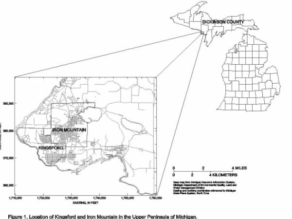
The cities of Kingsford and Iron Mountain are in the southwestern part of
Dickinson County in the Upper Peninsula of Michigan. Residents and businesses
in these cites rely primarily on ground water from aquifers in glacial deposits.
Glacial deposits generally consist of an upper terrace sand-and-gravel unit
and a lower outwash sand-and-gravel unit, separated by lacustrine silt and clay
and eolian silt layers. These units are not regionally continuous, and are absent
in some areas. Glacial deposits overlie Precambrian bedrock units that are generally
impermeable. Precambrian bedrock consists of metasedimentary (Michigamme Slate,
Vulcan Iron Formation, and Randville Dolomite) and metavolcanic (Badwater Greenstone
and Quinnesec Formation) rocks. Where glacial deposits are too thin to compose
an aquifer usable for public or residential water supply, Precambrian bedrock
is relied upon for water supply. Typically a few hundred feet of bedrock must
be open to a wellbore to provide adequate water for domestic users. Ground-water
flow in the glacial deposits is primarily toward the Menominee River and follows
the direction of the regional topographic slope and the bedrock surface.
To protect the quality of ground water, Kingsford and Iron Mountain are developing
Wellhead Protection Plans to delineate areas that contribute water to public-supply
wells. Because of the complexity of hydrogeology in this area and historical
land-use practices, a steady-state ground-water-flow model was prepared to represent
the ground-water-flow system and to delineate contributing areas to public-supply
wells. Results of steady-state simulations indicate close agreement between
simulated and observed water levels and between water flowing into and out of
the model area. The 10-year contributing areas for Kingsford's public-supply
wells encompass about 0.11 square miles and consist of elongated areas to the
east of the well fields. The 10-year contributing areas for Iron Mountain's
public-supply wells encompass about 0.09 square miles and consist of elongate
areas to the east of the well field.
In 1997, the U.S. Geological Survey, in cooperation with the cities of Kingsford
and Iron Mountain, began a 2-year study to describe ground-water flow and determine
the areas that contribute water to the cities' public-supply wells. The cities
of Kingsford and Iron Mountain are in the southwestern part of Dickinson County,
in the Upper Peninsula of Michigan (fig. 1).
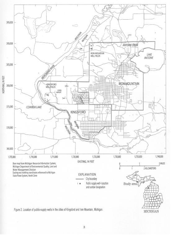
Both of these cities currently have four municipal wells in glacial aquifers
that provide ground water to residents and businesses for water supply (fig.
2). In an effort to protect the quality of ground water that is withdrawn
by these wells, the cities of Kingsford and Iron Mountain are developing Wellhead
Protection Plans (WHPP). As part of WHPP, the cities will delineate areas that
contribute water to public-supply wells. Kingsford's wells are located near
Cowboy Lake and near Ford Airport (fig. 2).
Iron Mountain's wells are located about 2 miles north of Kingsford's well fields.
Because of the complexity of hydrogeology in these areas and historical land-use
practices, a computer model is needed to describe the ground-water-flow system
and to delineate areas that contribute water to public-supply wells.
This report describes the hydrology of the Kingsford-Iron Mountain area and
the simulation of ground-water flow in the Kingsford-Iron Mountain area. During
this study, water levels were measured in 28 domestic, irrigation, and observation
wells to determine ground-water-flow directions. Thirteen aquifer tests performed
previously to this study were reanalyzed and one aquifer test was conducted
during this study to determine hydraulic conductivity information for the ground-water-flow
model. Particle-tracking analysis was used in conjunction with flow simulations
to delineate the land surface and subsurface areas that contribute water to
the public-supply wells. Model simulations are based on the U.S. Geological
Survey Modular Three-Dimensional Finite-Difference Ground-Water Flow Model,
MODFLOW-96 (McDonald and Harbaugh, 1988, 1996), which is a generalized code
for ground-water-flow modeling. Areas contributing water to supply wells were
determined using a particle-tracking post-processor package for MODFLOW (MODPATH,
Pollock, 1989).
Figure 1. Location of Kingsford and Iron Mountain in the Upper Peninsula of Michigan.
Figure 2. Location of public -supply wells in the cities of Kingsford and Iron Mountain, Michigan.
Numerous studies have contributed to an understanding of the geology and hydrology
of this area. Kingsford and Iron Mountain have evaluated potential areas for
well-field development. These evaluations include test borings, aquifer tests,
and geophysical surveys (Keck Consulting Services, Inc., 1974; Coleman Engineering
Co., 1975, 1980, 1982, and 1987; Lynn M. Miller, P.E., 1976; Sundberg, Carlson,
and Associates, Inc., 1989; and McNamee, Porter and Seeley, 1981 and 1990).
Two studies in the area (Engineering for Earth, Water, and Air Resources [EWA],
1986; 1987) focused on hydrogeologic conditions at a site in Kingsford that
was used for manufacturing facilities. In this area, glacial kettles (depressions
in the land surface formed by melting of ice blocks and subsidence of overlying
deposits) were used as retention ponds for waste products. EWA's investigations
included installation of monitoring wells and soil borings, and development
of a ground-water-flow model to determine the potential effect of these waste-disposal
pits on water quality, and the potential effect on Kingsford's water supply.
Subsequent investigations have been conducted and indicate that although environmental
contamination is present near historic industrial sites, it is unlikely that
these areas pose any threat to the quality of water at either the Kingsford
or Iron Mountain well fields.
The authors gratefully acknowledge the assistance of Darryl Wickman, Tony Edlebeck,
George Groeneveld, and Al Muntz, city of Kingsford; and Jim Urbany and John Ellis, city of Iron Mountain, for providing information and access to the public-supply wells and providing other sources of information about the cities; Chuck Thomas, Drinking Water and Radiological Protection Division, Michigan Department of Environmental Quality, for providing copies of reports and information about geologic and hydrologic conditions in the areas; and Shirley Businski, Land and Water Management Division, Michigan Department of Environmental Quality, for providing information on public-supply wells. Sincere thanks also are given to homeowners and golf course owners, who permitted access to their wells for water-level measurements.
The cities of Kingsford and Iron Mountain are bounded by the Menominee River to the south and west, and by Trader Hill to the north (fig. 2). The Kingsford-Iron Mountain study area is within the Menominee River drainage basin which includes Dickinson County, Mich. and Florence County, Wisc. Historically, iron ore and timber industries were important to the area, while currently lumber and paper industries, tourism, and recreational activities support the area's economy. The geologic and hydrologic characteristics that affect ground-water flow in the study area are described below.
Most of the Kingsford-Iron Mountain area is underlain by Precambrian metasedimentary
(Michigamme Slate) and metavolcanic (Badwater Greenstone and Quinnesec Formation)
rocks. The Michigamme Slate consists of fine- to medium-grained metagraywacke
and slate in massive or graded beds, whereas the Badwater Greenstone consists
of massive, chloritized mafic volcanic rocks (Sims, 1990). The Quinnesec Formation
consists of mafic and felsic volcanic rocks (Oakes and others, 1973). In the
vicinity of Pine Mountain, Millie Hill, and Trader Hill (fig.
3), bedrock consists of metasedimentary rocks of the Vulcan Iron Formation,
with alternating iron-rich and quartz-rich layers, and the Randville Dolomite,
consisting of massive dolomite with detrital quartz grains and thick-bedded
crystalline dolomite (Sims, 1990).
Bedrock is overlain by Pleistocene glacial deposits, except where bedrock is
exposed along the Menominee River to the south and to the north near Spread
Eagle, Wisconsin (Clayton, 1986). There also are isolated areas where bedrock
is exposed (for example, Ford Airport), but these are of small areal extent.
Glacial deposits range from 0 to about 380 ft in thickness. The Marenisco Moraine
(Martin, 1955) forms a distinct ridge through the Kingsford-Iron Mountain area
(fig. 3). Approximately parallel to this
moraine and south of the Menominee River lies another moraine informally referred
to as the Menominee Moraine.
Within the study area, glacial deposits generally consist of an upper terrace
sand-and-gravel unit and a lower outwash sand-and-gravel unit separated by intermediate
lacustrine silt and clay and eolian-silt layers (figs. 4,
5, and 6).
These units are not regionally continuous and are absent in some isolated areas
within Kingsford as indicated by boring logs. Towards the west and north, information
obtained from well and geophysical logs indicates that upper terrace and lower
outwash sand-and-gravel units are separated primarily by silt and fine sand.
The upper sand-and-gravel unit ranges from 0 to 160 ft in thickness and consists
of medium to fine-grained sand with varying amounts of silt and gravel (Engineering
for Earth, Water, and Air Resources, Inc., 1987). The confining unit ranges
from 0 to 150 ft in thickness and consists of well sorted and well compacted
fine silt and clay. In some areas, the silt and clay are absent, possibly due
to partial burial and protrusion of stranded ice blocks that prevented silt
deposition (Engineering for Earth, Water, and Air Resources, Inc., 1987). The
lower sand-and-gravel unit ranges from 0 to 237 ft in thickness and consists
of moderately well sorted fine to coarse sand with layers and lenses of silt
and gravel (Engineering for Earth, Water, and Air Resources, Inc., 1987). The
lower sand-and-gravel unit is underlain by a lodgement till or the Vulcan Iron
Formation over much of the area. The lodgement till and Vulcan Iron Formation
units range from 0 to 250 ft in thickness. West of the Menominee River, glacial
deposits consist primarily of till or fluvial sediments that change conspicuously
within relatively short distances (Clayton, 1986). The sediments consist of
sand and gravel, which were deposited by glacial melt-water streams. The till
consists of reddish brown or dark brown gravelly sandy loam with abundant surface
boulders (Clayton, 1986, plate 1).
Figure 3. Location of well fields and physical featues in the Kingsford-Iron Mountain area, Michigan
Precipitation averages about 29 in/yr over the Kingsford-Iron Mountain area.
Mean monthly precipitation ranges from a minimum in February of 0.9 in to a
maximum in August of 3.7 in. The study area receives about 62.8 in/yr of snowfall
(Midwestern Climate Center, 1999). Precipitation averages about 30 in/yr in
the Pine-Popple River Basin, west of the Menominee River, and is highest from
late spring to early autumn (Oakes and others, 1973).
Two glacial aquifers (upper and lower aquifers) underlie the study area, based
on previous studies and available well and boring logs. The upper aquifer in
the glacial deposits consists of the upper terrace sand-and-gravel unit, whereas
the lower aquifer in the glacial deposits consists of the lower outwash sand-and-gravel
unit. The intermediate silt layer is a fairly effective barrier to hydraulic
communication between the two aquifers. This lack of hydraulic communication
is strongly indicated by substantial head differences between the two aquifers;
water levels in shallow wells typically are 20-60 ft higher than water levels
in deep wells (D.B. Westjohn, oral commun., 2000). Where the silt layer is absent
in the Kingsford area, the upper and lower sand-and-gravel units compose one
aquifer (Engineering for Earth, Water, and Air Resources, Inc., 1987). Hydraulic
conductivities for the upper aquifer in the Kingsford area range from 9 to 0.9
ft/d based on tests performed by Engineering for Earth, Water, and Air Resources,
Inc. (1987). Hydraulic conductivities average about 9 ft/d for the lower aquifer
and range from 0.001 to 0.5 ft/d for the intermediate confining unit (Engineering
for Earth, Water, and Air Resources, Inc., 1987).
An understanding of the hydraulic characteristics of glacial aquifers in the
public-supply well field areas has been obtained from aquifer tests performed
during investigations of potential areas for well-field development (fig.
2, table 1). Aquifer tests of wells in the lower aquifer
indicate ground-water leakage from overlying units. Iron Mountain's Well #4
is screened within the lower aquifer; however, in the immediate area surrounding
well #4 the upper aquifer is missing.
Ground-water flow within the Kingsford-Iron Mountain area is primarily towards
the surface-water bodies to the west and southwest and follows the topographic
slope and the bedrock surface. Generally, the topographic slope follows the
bedrock surface except within the central part of Kingsford where there is a
bedrock low. Ground-water flow is probably confined primarily within the permeable
sand-and-gravel units because Precambrian bedrock units appear to be largely
unfractured and limit downward migration of ground water. However, bedrock consists
of metasedimentary rocks in the vicinity of Pine Mountain and Millie Hill, and
ground-water flow is locally controlled by these units where they are fractured.
The conceptual model describes ground-water flow within the Kingsford-Iron
Mountain and surrounding areas and includes a definition of the position and
thickness of aquifer and confining units, boundaries, and the flow system. Geologic
units within the Kingsford-Iron Mountain area can be divided into layers that
control ground-water flow.
Four units were used to conceptualize the ground-water-flow system although
not all units are present throughout the study area. These units consist of
an upper permeable sand-and-gravel unit, an underlying confining unit consisting
of silt and clay, a lower permeable sand-and-gravel unit, and a lowermost unit
consisting of sandstone, dolomite, or lodgement till (where they are present).
The bedrock of the Vulcan Iron Formation and the Randville Dolomite and the
lodgement till of the glacial unit are poorly permeable and were combined in
the lowermost unit because of their similar hydraulic properties.
Although these units are poorly permeable, some domestic wells withdraw water
from the bedrock; however, a few hundred feet of borehole must be open to a
wellbore to provide an adequate supply. Geologic information obtained from logs
of public-supply and domestic wells and geophysical logs were used to delineate
the extent of the ground-water-flow system units.
Ground-water-flow systems have physical boundaries, which are formed by the
presence of an impermeable body of rock or a large body of water, or hydrologic
boundaries, which include ground-water divides and streamlines. Regional physical
boundaries to the flow system are formed by the boundaries of the Menominee
River drainage basin that extends west into Wisconsin and east into Michigan.
Boundaries for the local-flow system in the Kingsford-Iron Mountain area consist
primarily of bedrock and surface-water bodies in Michigan and Wisconsin that
affect flow to the Menominee River. Locally, ground-water flow is affected by
physical boundaries formed by bedrock highs south of the Menominee River and
north of Iron Mountain's well fields, and by surface water bodies including
Lake Antoine on the east, and the Pine and Little Popple Rivers on the west.
Ground-water-flow divides are assumed to coincide with the surface-water divides
which follow topographic highs and the impermeable bedrock in this area. Local
hydrologic boundaries consist of streamlines, which are perpendicular to the
ground-water-flow direction along the east and northeast. The lower boundary
is formed by the upper surface of the Michigamme Slate, Badwater Greenstone,
and Quinnesec Formations and is considered to be poorly permeable.
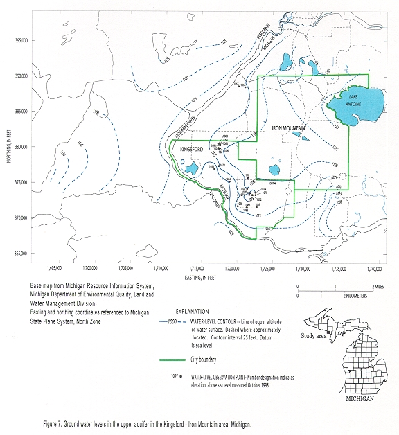
A preliminary understanding of ground-water-flow directions can be made on the
basis of surface-water elevations taken from topographic maps of the area, ground-water
levels measured during this study, and previous reports covering part of the
study area. For this study, water levels were measured in 28 domestic, irrigation,
and observation wells. Water levels recorded on well logs and average drawdown
measurements obtained for each of the public-supply wells also were analyzed
to understand ground-water-flow directions. Regional ground-water flow is towards
the Menominee River and follows the direction of the regional topographic slope
and the bedrock surface (fig. 7).
Figure 7. Ground water levels in the upper aquifer in the Kingsford - Iron Mountain area, Michigan
SIMULATION OF GROUND-WATER FLOW
Simulation of ground-water flow is made possible by first developing a conceptual model of the flow system and then developing a numerical model that is consistent with the conceptual model. The model area consists of the Kingsford-Iron Mountain area and surrounding parts of Dickinson County, Michigan and Florence County, Wisconsin. This larger area (larger than the cities of Kingsford and Iron Mountain) was modeled so as to eliminate boundary effects on the ground-water-flow solution in the interior portion of the model area by allowing natural physical and hydrologic boundaries to be chosen, as well as to investigate whether ground water moved beneath the Menominee River as possibly indicated by the high change in ground-water levels from Pine Creek to the Menominee River.
Numerical Model
The U.S. Geological Survey Modular Three-Dimensional Finite-Difference Ground-Water
Flow Model (MODFLOW-96, McDonald and Harbaugh, 1996) was the computer code used
to simulate ground-water flow in the Kingsford-Iron Mountain area.
This code allows the simulation of steady-state ground-water flow in two dimensions
with leakage between model layers; no ground-water storage or temporal discretization
terms are required. All water entering the model area through the boundaries
or as recharge is assumed to leave the model area through the boundaries, rivers,
or wells. The Kingsford and Iron Mountain wells have been in operation for 8
to 25 years; therefore the ground-water flow system is considered to be in steady
state and water is not lost or gained from storage.
Various assumptions were made in the numerical simulation of ground-water flow.
Recharge to ground water was assumed to differ over the model area depending
on the presence or absence of glacial till. Recharge is assumed to be zero in
areas where till or bedrock is at or very near the surface. In other areas recharge
initially was assumed to be 10 in/yr. The assumption of no recharge to areas
of till and bedrock highs was investigated during model calibration. Evapotranspiration
of ground water also was assumed to be zero because recharge was applied to
the upper surface of the model (water table), where the effects of evapotranspiration
are expected to be small, and because of the regional scale of the model. Ground
water was assumed to flow primarily through the glacial sand-and-gravel units.
Glacial deposits are known to vary considerably with varying lithologies and
thicknesses over short distances. This variability makes exact representation
of the detailed hydrogeology impossible in the numerical model. Thus, hydraulic
properties of the glacial deposits are generalized to represent the regional
ground-water-flow system. The underlying lodgement till and bedrock units of
the Vulcan Iron Formation and Randville Dolomite were simulated as a low permeability
layer. The lowermost Precambrian bedrock units were simulated as impermeable
boundaries. North of the Chapin Mine, ground water is withdrawn from thHamilton
Mine Shaft that extends deep into the underlying bedrock units and is discharged
into Lake Antoine (fig. 3). A probable hydraulic
connection is present between the bedrock and Lake Antoine based on that water
levels in the mine shaft only can be lowered approximately 2 feet even with
extensive pumping and the high gradient from the lake to the shaft. It is possible
that the withdrawal of ground water from this mine shaft affects local ground-water
levels in the immediate vicinity; however, this area is over 1.5 mi from the
public-supply well fields and is not thought to affect hydrologic conditions
there. Therefore, these conditions were not simulated in the model.
Model Grid and Layers
The modeled area is rectangular and consists of about 64 mi2 (fig.
8). The area is 6.7 mi long (north-south) and 9.5 mi wide (east-west). This
area is horizontally discretized into a variably spaced grid of cells in 213
columns and 204 rows. In the central portion of the model, each cell is 100
by 100 ft. Cell spacing increases initially by a factor of 1.25 for 5 rows/columns
and then by a factor of 1.5 out to a maximum grid spacing of 1,029 ft. This
maximum spacing was selected so as not to exceed a maximum row to column spacing
ratio of 10:1. Each grid cell represents the average aquifer properties in the
volume of aquifer represented by the cell; any variations in properties that
are within a grid cell only can be represented in the model averages.
The model area is vertically discretized into three
model layers. Layer 1 represents the upper aquifer in the glacial deposits.
This aquifer is under unconfined conditions with water levels representing the
water table. Layer 2 represents the lower aquifer in the glacial deposits. The
lower aquifer represented in layer 2 is simulated as convertible and can be
either confined or unconfined depending on the position of the water table.
The intermediate confining unit that separates the upper and lower aquifers
was included only in the leakance term between layers 1 and 2. The bottom model
layer (layer 3) represents either metasedimentary rocks (in the vicinity of
Pine Mountain, Millie Hill, and Trader Hill) or lodgement till (over the remaining
area) and also is represented as convertible.
| Model layer | Hydrologic unit |
|---|---|
| 1 | Upper aquifer in glacial deposits |
| 2 | Lower aquifer in glacial deposits |
| 3 | Lodgement till/ metasedimentary rocks |
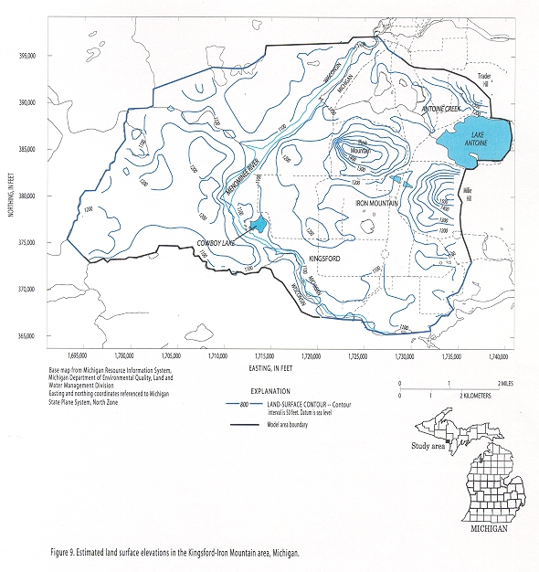
Land-surface information for most of the model area is available from a digital
1:100,000 topographic quadrangle map for Iron Mountain. This information was
interpolated to a grid with a 50 ft spacing. Additional point-altitude data
were taken from the topographic quadrangle map for Iron Mountain SW. This information
was contoured over the model area to create land-surface elevations, which constitute
the top of glacial deposits (fig. 9). The
land surface is characterized by steep gradients in the vicinities of Pine Mountain,
Millie Hill, and Trader Hill.
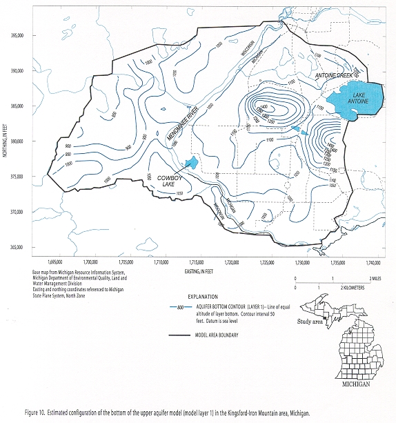
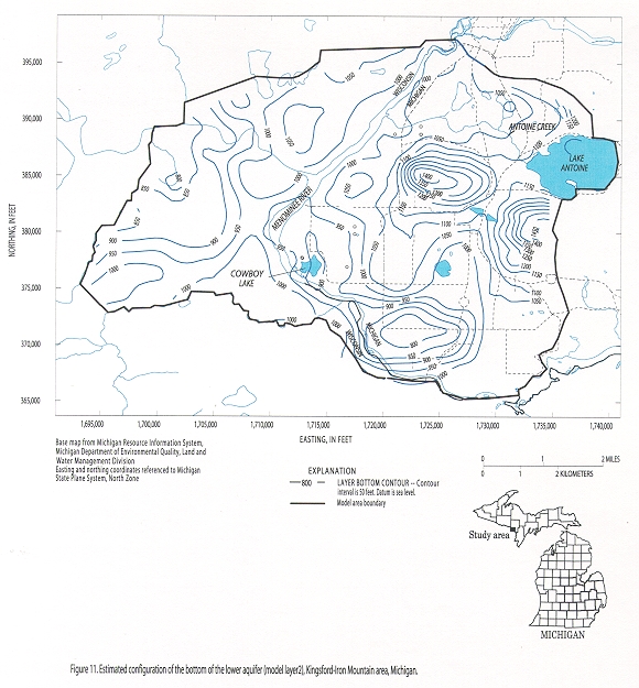
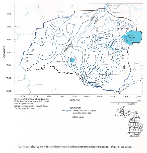
Layer surfaces were determined based on logs of domestic and public-supply wells
obtained from Geological Survey Division, Michigan Department of Environmental
Quality; Statewide Ground-Water Database, MIRIS-Geologic Resource Mapping Unit,
Michigan Department of Environmental Quality; and Wisconsin Geologic and Natural
History Survey (figs. 10, 11,12).
The top of the silt unit formed the bottom of layer 1 and the silt unit thickness
was assigned to layer 2. In areas where the geologic materials composing a layer
are absent, the layer is assigned a minimal thickness and the hydraulic properties
of the overlying layer. Information for the Wisconsin part of the model area
did not differentiate the glacial deposits into separate vertical units; therefore,
on the western side of the Menominee River, glacial deposits are modeled as
the upper layer with layer 2 assigned a 1 ft thickness and the hydraulic conductivity
of the overlying layer. Additional delineation of layer surfaces in areas of
sparse data was done by extrapolating from known nearby points, primarily within
Wisconsin where few well logs are available. In the vicinity of Pine Mountain,
Millie Hill, and Trader Hill, till overlies the bedrock units and the sand-and-gravel
units are missing. Outcrops provide additional control for the delineation of
the bedrock surface, especially in Wisconsin where outcrops indicate that glacial
deposits are thin.
Figure 9. Estimated land surface elevations in the Kingsford-Iron Mountain area, Michigan.
Figure 10. Estimated configuration of the
bottom of the upper aquifer model (model layer 1)
in the Kingsford-Iron Mountain area, Michigan.
Figure 11. Estimated configuration of the bottom of the lower aquifer (model layer 2), Kingsford-Iron Mountain area, Michigan
Model boundaries extend approximately 1 mi north of the Iron Mountain well
field, approximately 1 mi south of the Kingsford well field, and approximately
2 mi east and 3 mi west of the well fields (fig.
8). These boundaries are based on surface-water elevations and topographic
information, and are represented by specified head, specified flux, and head-dependent
flux conditions. Specified head boundaries (also referred to as constant head
boundaries) are modeled by specifying head values that do not change during
numeric simulation. Specified flux boundaries can be modeled by specifying the
flux equal to zero to represent ground-water-flow divide boundaries and streamlines.
Head-dependent flux boundaries are modeled by specifying a conductance, which
limits the amount of water that can enter or leave any cell.
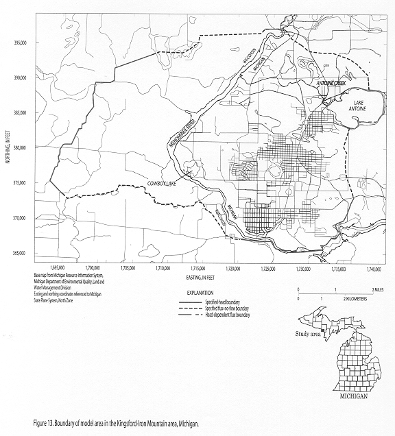
Specified head boundaries are used to represent hydraulic conditions along parts
of the east and west model boundaries and are based on surface-water elevations
(fig. 13). Specified head boundaries also
were used to represent the southernmost part of the Menominee River. Specified
flux boundaries with flux equal to zero are used to represent natural physical
boundaries formed by outcropping or shallow bedrock along parts of the north
and south model boundaries. Specified flux boundaries with flux equal to zero
also are used to represent ground-water-flow divides and streamlines along parts
of the north and west boundaries. Finally, head-dependent flux boundaries are
used to represent Lake Antoine along part of the east boundary and three small
lakes along the west boundary.
In areas where a natural physical boundary does not exist, specified head boundaries
located far from the well fields were used, based on available water-level data.
After model development, sensitivity of model results to boundary conditions
were analyzed. Fluxes through cells forming specified head boundaries were compared
for simulations in which public-supply wells were being pumped and when wells
were idle. As an additional check on the ground-water-flow solution, specified
head boundaries were changed to specified flow boundaries and the solutions
compared. The effect of stresses induced by pumping (on the assumption of no-flow
across streamlines) also was investigated.
All boundaries of layer 2 are the same as those of layer 1, except that no-flow
boundaries are located in the area of Lake Antoine, because the lake does not
penetrate the lower sand-and-gravel unit. Layer 3 is bounded by no-flow boundaries.
In layers 1 and 2, the Chapin Mine area of the model is represented by inactive
(no-flow) cells and by head-dependent flux cells in layer 3. In this area, glacial
deposits are relatively thin and unsaturated, and ground water is present only
in the bedrock unit below the glacial deposits.
Figure 12. Estimated configuration of the bottom of the lodgement till and metasedimentary rocks (model layer 3), Kingsford-Iron Mountain area, Michigan
Figure 13. Boundary of model area in the Kingsford-Iron Mountain area, Michigan.
Hydraulic properties used in model simulations include layer hydraulic conductivities
and leakances, recharge rates, and streambed conductance. Aquifer hydraulic
properties and leakances affect ground-water flow through and between model
layers. Recharge rates indicate the amount of water movement through the upper
surface of the model. Streambed conductance affects vertical flow of ground
water from an aquifer to a stream or from a stream to an aquifer.
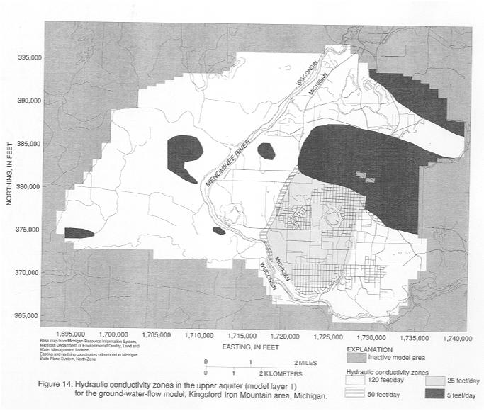
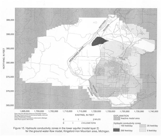
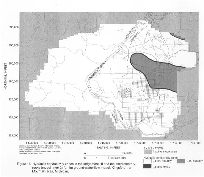
Based on interpretation of well and geophysical logs, eleven zones were used
to describe conditions within the three layers (table 2,
figs. 14, 15,
16). The upper and lower aquifers were
separated into different zones based on calculated horizontal hydraulic conductivities
from aquifer-test analyses. Transition zones were added to reduce the difference
in hydraulic conductivities between zones in some areas. Initial estimates of
hydraulic conductivity for the zones within each layer were based on calculated
hydraulic conductivities from aquifer-test analyses and on representative values
estimated by Freeze and Cherry (1979) for the geologic materials present in
the area.
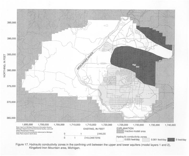
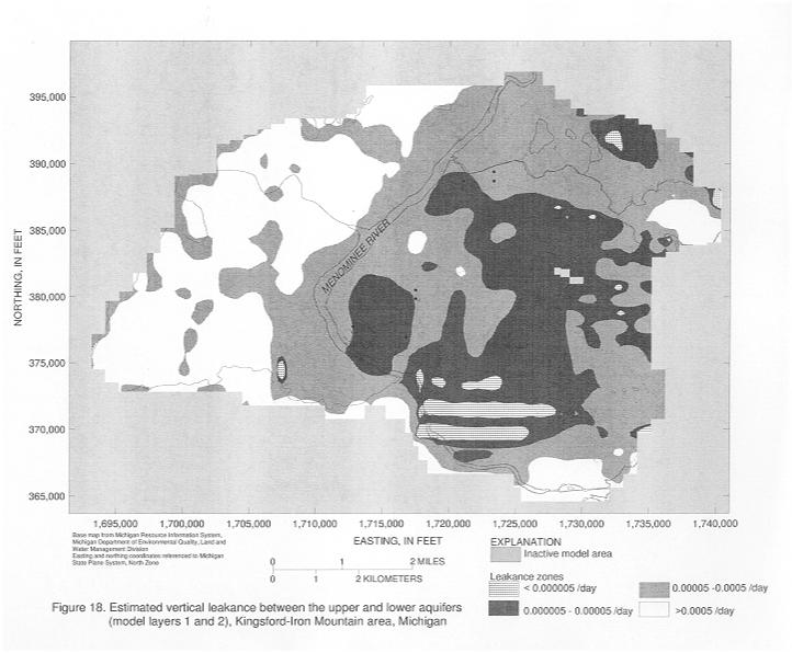
Leakances as described by McDonald and Harbaugh (1988) are based on the layer
thicknesses and the vertical hydraulic conductivity for each layer. The initial
estimate of leakance between layers 1 and 2 was based on the thickness and assigned
values for the hydraulic conductivity of the confining unit that separates the
upper and lower aquifers. Vertical hydraulic conductivities were assigned based
on the type of geologic materials present and consisted of zones representing
till in the vicinity of Pine Mountain and Millie Hill, silt and clay in the
south Kingsford area and to the north near Iron Mountain Well #4, and silt and
silty sand over the rest of the area (fig.
17). These vertical hydraulic conductivities then were divided at each grid
cell location by the layer thickness. The resulting values for leakance between
layers 1 and 2 ranged from 3.8x10⁻⁶ to 2.5x10⁻³ /d (fig.
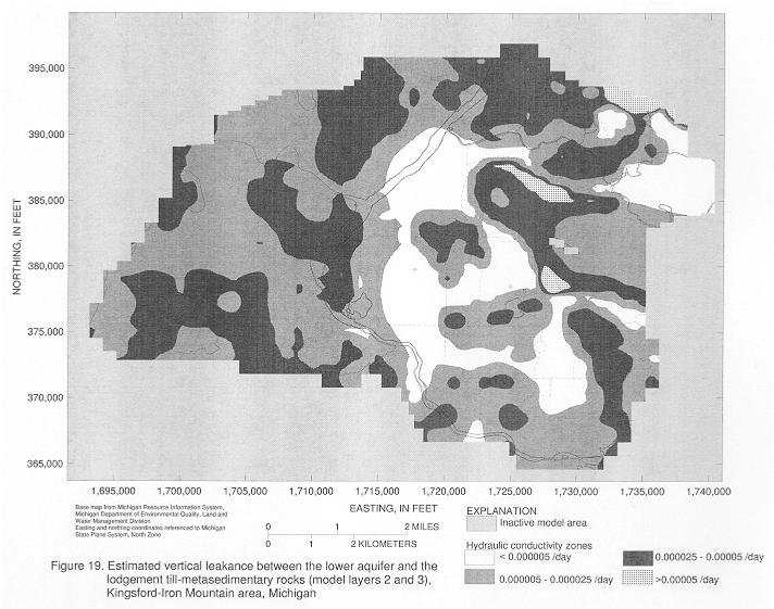
18). The initial estimate of leakance between layers 2 and 3 was based on
the vertical hydraulic conductivity of the geologic materials present and the
thickness of the over- and underlying layers. The resulting values for leakance
between layers 2 and 3 ranged from 1.8x10⁻⁷ to 4x10⁻³ /d (fig.
19). Initial estimates of vertical hydraulic conductivity were assumed to
be 0.01 times the horizontal hydraulic conductivity for each zone.
Figure 14. Hydraulic conductivity zones in the upper aquifer (model layer 1) for the ground-water-flow model, Kingsford-Iron Mountain area, Michigan.
Figure 15. Hydraulic conductivity zones in the lower aquifer (model layer 2) for the ground-water-flow model, Kingsford-Iron Mountain area, Michigan.
Figure 16. Hydraulic conductivity zones in the lodgement till and metasedimentary rocks (model layer 3) for the ground-water-flow model, Kingsford-Iron Mountain area, Michigan.
Figure 17. Hydraulic conductivity zones in theconfining unit between the upper and lower aquifers (model layers 1 and 2) Kingsford-Iron Mountain area, Michigan.
Figure 18. Estimated vertical leakance between the upper and lower aquifers (model layers 1 and 2), Kingsford-Iron Mountain area, Michigan.
Figure 19. Estimated vertical leakance between the lower aquifer and the lodgement till-metasedimentary rocks (model layers 2 and 3), Kingsford-Iron Mountain area, Michigan.
Recharge was assumed to differ in areas depending on the type and thickness
of glacial deposits and was applied to the top model layer. In areas of surficial
till, and in areas where the bedrock is located near the land surface, recharge
was assumed to be zero. Over the rest of the area, recharge initially was assigned
a value of 10 in/yr. Estimates of average discharge obtained from three nearby
U.S. Geological Survey (USGS) gaging stations equaled 18.3 in/yr from 191to
1996 for the Menominee River near Florence, Wisc. (USGS gaging station 04063000);
15.1 in/yr from 1914 to 1997 for the Menominee River at Twin Falls near Iron
Mountain, Mich. (USGS gaging station 04063500); and 13.8 in/yr from 1993 to
1997 for the Menominee River at Niagara, Wisc. (USGS gaging station 04065106,
Water Resources Data for Michigan, Water Years 1996 and 1997). These discharges
represent an upper limit for recharge because they include both baseflow and
runoff. Actual estimates of baseflow could not be determined because of the
presence of numerous control structures along the Menominee River.
In MODFLOW (McDonald and Harbaugh, 1988), streambed conductance is calculated
as the product of the hydraulic conductivity of the streambed materials, stream
length, and stream width, divided by the streambed thickness. Stream lengths
for cells representing the Menominee River were equal to the length of the cell
(fig. 8). Stream widths were assumed to
be equal to approximately 100 ft. Stream lengths for cells representing the
Pine River, Pine Creek, and Little Popple River in Wisconsin were equal to the
length of the cell. Stream widths were assumed to equal 10 ft except along one
section of the Pine River where the width was assumed to equal 100 ft. Stream
lengths and widths for cells representing Antoine Creek were assumed to be 10
ft. Streambed thicknesses were assumed to be 1 ft. Hydraulic conductivities
of the streambed materials were initially assigned a value of 10 ft/d, except
for the section of Antoine Creek in the area immediately north of Iron Mountain
Well #3 which was assigned an initial value of 1 ft/d. In this area, Coleman
Engineering Company (1980) observed that the creek bottom consisted of silty
sand which limits the direct flow of water from the creek to the well at this
location. Horizontal hydraulic conductivities for the lake cells were initially
estimated to be 10 ft/d.
Ground-water withdrawals were simulated from the center of the cell containing
a pumping well. Because of the close proximity of Iron Mountain wells 1 and
2, these wells were simulated as pumping from the same cell. Withdrawals from
Kingsford and Iron Mountain wells totaled:
| 0.76 mgd | Iron MountainWells #1 and #2 |
| 0.14 mgd | Iron Mountain Well #3 |
| 0.32 mgd | Iron Mountain Well #4 |
| 0.15 mgd | Kingsford Well #1 |
| 0.28 mgd | Kingsford Well #5 |
| 0.23 mgd | Kingsford Well #6 |
| 0.37 mgd | Kingsford Well #7 |
Model calibration is the process of reducing the difference between measured
and simulated water levels and flows by adjusting model parameters. Multiple
calibration trials were used to determine the set of parameter values that produced
the best fit between simulated and measured values, whereas keeping parameters
and the overall water budget within estimated values.
Head data used in the calibration of the ground-water-flow model include water-level
measurements made during this study, measurements made during previous investigations
of the Kingsford area, and measurements recorded on domestic well logs. Of the
measurements used for this study, 24 are in layer 1, 44 are in layer 2, and
5 are in layer 3. Long-term drawdown measurements for the public-supply wells
were included for comparison purposes. Because of the way in which pumping is
represented in the model (continuous pumping at a constant rate, rather than
intermittent pumping at varying rates); however, the water-level measurements
at pumping wells will not be represented exactly.
Flow data at USGS gaging stations were examined to determine upper and lower
bounds on flow within the Menominee River. Long-term data (greater than 80 years
of record) are available for two stations (04063000 and 04063500) on the Menominee
River upstream of the model area. Flow at these stations averaged 1,797 ft3/s
for 04063000 and 1,812 ft3/s for 04063500 over the available years of record
for similar size drainage basins (Water Resources Data for Michigan, Water Years
1996 and 1997). The length of river reach between these two stations is approximately
the same length as that in the model area and the flow is assumed to be representative.
The difference between these flows is small and is probably within the expected
error range of the measurements; however, this comparison serves to illustrate
that flow to river cells within the model is expected to be small (less than
15 ft3/s).
Model sensitivity was investigated by varying model parameters within expected
ranges (scenarios 1 - 9, Appendix) and comparing the resulting root mean square
errors (RMSE). Different scenarios were considered because of the complexity
of the ground-water system being represented, differing geologic materials and
water levels observed at adjacent wells, the steep gradients present, and the
unknown location of the water table in some areas of the model. The root mean
square error is the average of the squared differences in measured and simulated
water levels. RMSE values and simulated model flow budgets were compared for
scenarios in which recharge to ground water; hydraulic conductivity of the streambed
materials, zone 1 in layer 1, Cowboy Lake area, Iron Mountain Well #4 area,
and zone 5 in layer 2, and all zones in layer 3; and the leakances between layers
were varied. The best fit between measured and simulated water levels was achieved
when the Menominee River was represented as specified head cells in both layers
1 and 2 (scenario 1); however, this representation of the river does not allow
for the possibility of flow beneath the river which was investigated in other
scenarios (appendix).
The final parameter estimates (scenario 4) for each zone are within reasonable
ranges (table 3).
The horizontal hydraulic conductivities of layer zones are within the ranges
determined from aquifer tests and flow to river cells is within the expected
order of magnitude. Flow to river cells increased and water levels in layer
1 were higher with an increase in recharge. Recharge of 2 in/yr to till areas
did not change the extent of the unsaturated areas and water levels remained
about the same in all layers. Water levels in layer 1 were lower with increases
in hydraulic conductivity for layer 1 or 2. Water levels in layer 2 remained
about the same with an increase in the hydraulic conductivity of layer 1 and
decreased with an increase in the hydraulic conductivity of layer 2. Water levels
remained about the same with changes in the hydraulic conductivity of layer
3. Water levels were higher in layer 1 and remained about the same in layer
2 with changes in streambed hydraulic conductivity; however, flow to river cells
decreased with lower streambed conductivity and increased with higher streambed
conductivity. Changes in leakance resulted in small changes in water levels.
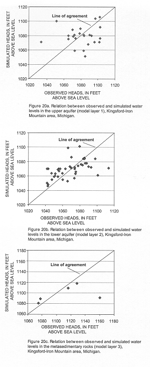
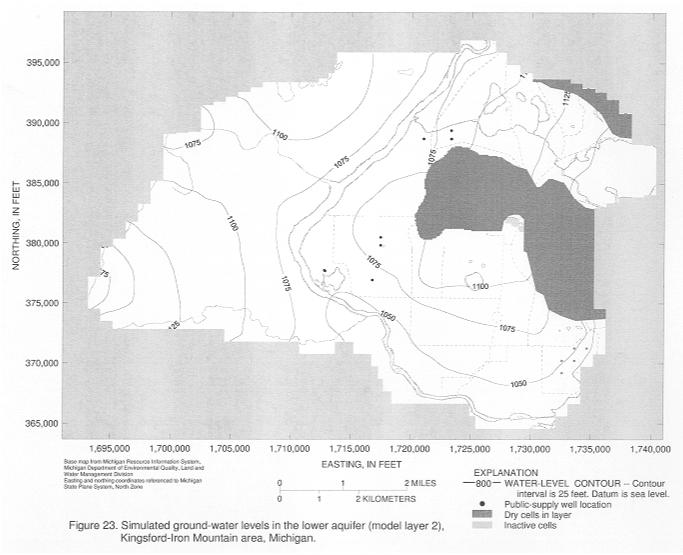
Results of model simulations indicate close agreement between water flowing
into and out of the model area; percent discrepancy equalled -0.49 (table
4). Generally simulated water levels are close to measured water levels
with the residuals about evenly split above and below the line representing
simulated equal to measured water levels (fig. 20a,
b, and c). Seventy-one percent of the simulated water levels are within
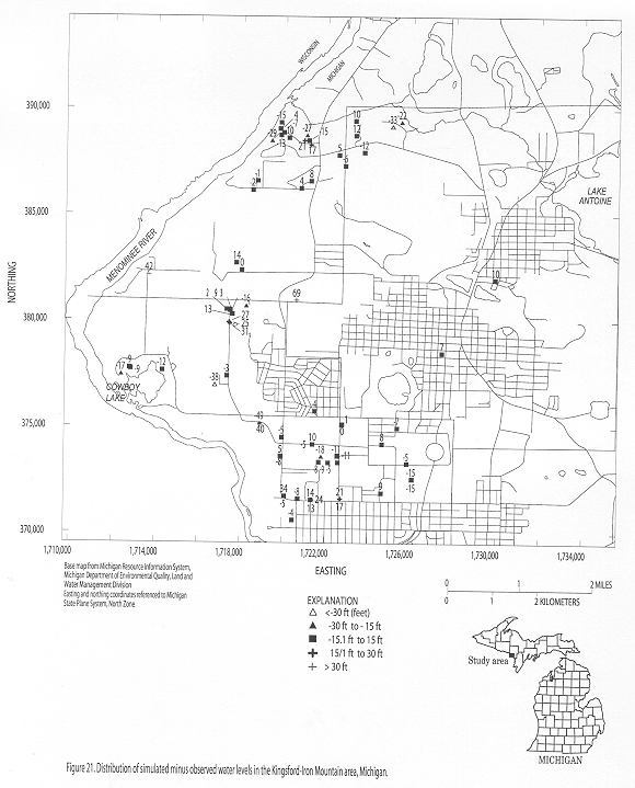
15 ft of the measured values. Differences between simulated and measured values
are shown in figure 21 and do not indicate any
spatial trends. Simulated water levels for layers 1 and 2 are shown in figures
22 and 23, respectively.
Part of the difficulty in matching measured values is due to large observed
differences in nearby wells. The simulated streamflow of 9.6 ft3/s is less than
15 ft3/s as expected. The simulated values obtained represent the best match
to these different values.
Figure 20a. Relation between observed and simulated water levels in the upper aquifer (model layer 1), Kingsford-Iron Mountain area, Michigan.
Figure 20b. Relation between observed and simulated water levels in the lower aquifer (model layer 2), Kingsford-Iron Mountain area, Michigan.
Figure 20c. Relation between observed and simulated water levels in the metasedimentary rocks (model layer 3), Kingsford-Iron Mountain area, Michigan.
Investigation of Boundary Effects
Choice of hydraulic boundaries (such as the specified heads used in this model) does not allow conditions along the boundaries to change from initial values; thus, one must investigate whether the boundaries are affecting the solution in the interior portion of the model (Anderson and Woessner, 1992). After selection of a final model, changes in conditions at boundaries were investigated by comparing flow through specified head cells forming boundaries for simulations in which wells were pumping and in which wells were idle. Flow through the individual specified head cells when the public-supply wells were pumping differed by an average of 2.6 percent (standard deviation equaled 23.8) from the flow through these same cells when the public-supply wells were simulated as idle. As an additional check on the boundaries, specified head cells were changed to specified flow cells using the well package to represent the specified flows. The ground-water-flow solution differed slightly near the edge of the dry cell area when the specified heads were changed to specified flows. Water-level differences between the two solutions at measurement locations were within 2 ft or less. Stresses induced from pumping by the public-supply wells only affected water levels locally and did not affect flow across streamlines.
The ground-water-flow model was developed to simulate the regional steady-state
response of the flow system in the Kingsford-Iron Mountain area to ground-water
withdrawals by the public-supply wells. Hydraulic properties in the aquifers
were assumed to be isotropic. (Within a cell hydraulic properties are the same
in the north-south direction as in the east-west direction;
hydraulic properties vary from location to location). Vertical variations in aquifer
properties within layers and any variations in head or flow within the aquifers
are not represented in the model. Model simulations are restricted to steady-state
conditions. All stresses within and inputs to the system, including well withdrawals
and recharge rates, remain constant throughout the simulation. No net gain or
loss of flow is simulated in the system and no changes in ground-water storage
occur. This model, in its current (2000) form, cannot be used to simulate transient-flow
conditions.
Each grid cell represents the average hydrologic and hydraulic properties in the
volume of aquifer represented by the cell, and any variations in properties within
the volume represented by the grid cell cannot be represented. Local flows over
distances smaller than the dimensions of the grid cell also cannot be accurately
represented. Additional geologic and hydrologic data, as well as finer discretization
of the model, would be needed to simulate smaller-scale flow systems. Hydraulic
properties of the individual layers are represented by zones and local variations
are not represented. This representation by zones generalizes the glacial and
bedrock properties and small-scale differences in ground-water flows are not represented.
This generalization was necessary because nearby wells often penetrate different
lithologic units with varying thicknesses and detailed geologic information is
unavailable for large portions of the model area. The accuracy of layer surfaces
and hydraulic conductivity estimates are limited by the available data at well
and boring locations. Additional control and accuracy could be achieved by inclusion
of more data points.
Recharge to ground water was assumed to vary over the model area depending on
the presence or absence of surficial till deposits and poorly permeable bedrock;
thus, local variations in recharge rates, such as those associated with impermeable
surfaces or differences in other types of surficial materials, are not represented
in the model. Recharge in areas of surficial till deposits is assumed to be negligible.
Simulated well withdrawals are assumed to come from the centers of grid cells.
Small withdrawals from domestic wells were not included because of the difficulty
in obtaining reliable data and the limitations in representing small-scale flow
systems. However, domestic ground-water withdrawals are probably small at the
scale of the model.
Other than flow within the Precambrian metasedimentary bedrock units in the vicinity
of Pine Mountain and Millie Hill, the model does not simulate flow within the
bedrock units. Thus, the bottom of the model is considered to be impermeable.
This assumption is considered adequate for model development because of the limited
flow available from fractures in bedrock. The model does not simulate flow through
fractures or fissures in the rocks. Primary and secondary porosities are combined
to represent average flow conditions. Thus, the presence of fractures and fissures
could create local heterogeneities in hydraulic properties, which can not be represented
by the model.
External boundary conditions were based on natural hydrologic conditions and were
located distant from Kingsford's and Iron Mountain's well fields, and, based on
the investigation of flow through the specified head cells, are assumed to have
minimal effect on the solution in the interior portion of the model. Enlargement
of the model area to natural physical hydrologic boundaries might improve model
simulations and convergence and improve the match between simulated and observed
ground water flows.
Different scenarios (in which recharge, hydraulic conductivity, and leakance parameters
were varied) were considered because of the complexity of the system, different
lithologic units and water levels observed at nearby wells, the steep gradients
present, and the unknown location of the water table in some parts of the model
area. Cells that went dry during model simulations were permitted to rewet; however,
most remained dry. Most of the dry cells were in the vicinity of Pine Mountain,
Millie Hill, and Trader Hill. In these areas the glacial deposits are thin and
unsaturated. The measured water level in a well drilled on top of Pine Mountain
shows that glacial deposits and bedrock are dry to the base of the mountain.
The accuracy of particle-tracking simulations is limited by the accuracy of the
numerical model on which the simulations are based, the estimates of the effective
porosity of the flow system, and the approximation of the cell flow velocities
to the local ground-water-flow velocities. Additionally, the particle-tracking
program considers ground-water flow by advection only. If the effects of dispersion
were included, the contributing areas could be larger. Because the model does
not specifically describe flow through fractures, ground-water flow and travel
times in areas where fractures are present may not be accurately represented.
Particle tracking was performed for public-supply wells near the center of the
model area. Detailed analysis of contributing areas for small localized areas
is inappropriate because the model was not designed to represent local flow systems.
The areas that are represented as being dry in model simulations may contribute
water and contaminants, if present, to the public-supply wells.
DELINEATION OF CONTRIBUTING AREAS
The particle-tracking program MODPATH (Pollock, 1989) can be combined with
MODFLOW-calculated flow in each cell to determine areas contributing water to
public-supply wells. In this study, the particle-tracking program was used by
specifying the locations of hypothetical water particles along the faces of
each cell containing a public-supply well. These particles then were tracked
backward in time through the ground-water-flow system until they reached the
top cell face in layer 1, which represents the starting location of the particle.
This collection of starting locations, projected up to the land surface, represents
the contributing areas for the public-supply wells. The subsurface zones through
which the particles travel are known as the zone of transport. Particles also
can be tracked for a specified amount of time, such as 10 years. This 10 year
time-of-travel area is identified by those particles whose travel times are
10 years or less. An estimated effective porosity of 15 percent was used in
the delineation for all layers. This value is less than the estimated total
porosity of 25 percent, which is representative of these types of materials
(Freeze and Cherry, 1996) and provides a conservative estimate of the contributing
areas. Particle tracking results were compared for several of the scenarios
and found to delineate similar areas.
Particle tracking describes the advective movement of ground water and does
not incorporate the effects of adsorption, diffusion, dispersion, and degradation.
Therefore, particle tracking is not intended as a substitute for modeling transport
of dissolved chemicals in a ground-water system.
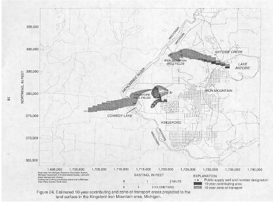
The 10-year contributing areas for Kingsford's public-supply wells encompass
about 0.11 mi2, or 302 model cells, and consist of elongated areas to the east
of the well fields (fig. 24). The 10-year
contributing areas for Iron Mountain's public-supply wells encompass about 0.09
mi2, or 30 model cells, and consist of elongated areas to the east of the well
field. The 10-year zone-of-transport consist of elongated zones east and west
of the well fields. Actual contributing areas may be larger because the areas
that are represented as being dry in model simulations may contribute water
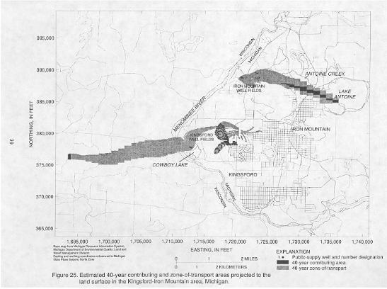
and contaminants, if present, to the public-supply wells. Forty year time-of-travel
contributing areas are shown in figure 25.
Figure 22. Simulated ground-water levels in the upper aquifer (model layer 1), Kingsford-Iron Mountain area, Michigan.
Figure 23. Simulated ground-water levels in the lower aquifer (model layer 2), Kingsford-Iron Mountain area, Michigan.
A ground-water-flow model was developed to simulate the regional, steady-state
ground-water flow system in the Kingsford-Iron Mountain area. Kingsford and
Iron Mountain are located in Dickinson County in the Upper Peninsula of Michigan.
These two cities rely entirely on ground water withdrawn for public supply from
the glacial deposits. The glacial deposits overlie Precambrian metasedimentary
(Michigamme Slate, Vulcan Iron Formation, and Randville Dolomite) and metavolcanic
(Badwater Greenstone) rocks, except along the Menominee River and in isolated
areas where bedrock is exposed. Glacial deposits range from 0 to about 380 ft
in thickness.
Two glacial sand-and-gravel aquifers are present in the study area. The upper
aquifer ranges from 0 to 160 ft in thickness and consists of medium to fine
grained sand with varying amounts of silt and gravel. The confining unit ranges
from 0 to 150 ft in thickness and consists of well sorted and well compacted
fine silt with clay. In some areas the silt and clay are absent due to partial
burial and protrusion of stranded ice blocks that prevented silt deposition.
The intermediate silt layer is a fairly effective barrier to hydraulic communication
between the two aquifers. However, where the silt is absent in the Kingsford
area, the two aquifers appear to be hydraulically connected. The lower aquifer
ranges from 0 to 237 ft in thickness and consists of moderately well sorted
fine to coarse sand with layers and lenses of silt. The lodgement till unit
ranges from 0 to 25 ft in thickness.
Ground-water flow within glacial deposits in the Kingsford-Iron Mountain area
is primarily towards surface-water bodies to the west and southwest and follows
the regional topographic slope and bedrock surface. Ground-water flow is probably
confined primarily within the permeable sand-and-gravel units because the Precambrian
bedrock units appear to be largely unfractured and limit the downward migration
of ground water. However, bedrock consists of metasedimentary bedrock units
in the vicinity of Pine Mountain, and ground-water flow is locally affected
by these units where they are fractured.
The ground-water-flow model developed for the Kingsford-Iron Mountain area encompasses
part of Dickinson County, Michigan and Florence County, Wisconsin. This area
is horizontally discretized into a variably spaced grid of cells in 213 columns
and 204 rows. The model area is vertically discretized into three model layers.
Layer 1 represents the upper aquifer in the glacial deposits; layer 2 represents
the lower aquifer in the glacial deposits; and layer 3 represents either lodgement
till or metasedimentary bedrock units where they are present in the model area.
The intermediate confining unit between the upper and lower glacial aquifers
is included only in the leakance term between layers 1 and 2. Specified-head,
specified flux, and head-dependent flux cells form the model boundaries.
Conceptualized estimates of hydraulic conductivity for each layer were based
on aquifer tests and on representative values taken from Freeze and Cherry (1979).
These estimates were modified during model calibration. Each of the three layers
was divided into zones containing similar geologic materials based on interpretation
of well and geophysical logs.
The model was calibrated using multiple trials where parameters were changed
to reduce differences between simulated and observed values, and to keep parameter
estimates and the overall model budget within reasonable limits. Differences
between observed and simulated values are attributed to the complex geology
and hydrology of this area, the steep gradients in the vicinities of Pine Mountain,
Millie Hill, and Trader Hill, and the large areas in which detailed hydrogeologic
information was unavailable. Different scenarios (in which recharge, hydraulic
conductivity, and leakance parameters were varied) were simulated in order to
verify the reproducibility of regional ground-water-flow directions and contributing
areas.
Contributing areas were delineated for Kingsford's and Iron Mountain's public-supply
wells using particle-tracking analysis. Results of flow simulations based on
1997-1998 pumping conditions indicate that 10-year contributing areas, delineated
by those particles with travel times of 10 years or less, cover 0.2 mi2.
| Table 1a. Root Mean Square Error (RMSE) values for selected scenarios[ft3/s, cubic feet per second; | |||||||||
|---|---|---|---|---|---|---|---|---|---|
| Parameter | Scenario 1 | Scenario 2 | Scenario 3 | Scenario 4 | Scenario 5 | Scenario 6 | Scenario 7 | Scenario 8 |
Scenario |
| Recharge | |||||||||
| till areas | 2 | 2 | 0 | 0 | 0 | 0 | 0 | 0 | 0 |
| rest of model area | 9 | 9 | 11 | 9 | 6 | 9 | 9 | 9 | 9 |
| Hydraulic conductivity | |||||||||
| Streambed materials | 0.02 | 0.04 | 0.1 | 0.04 | 0.02 | 0.02 | 0.04 | 0.04 | 0.04 |
| Most of layer 1 (zone 1) | 120 | 150 | 120 | 120 | 120 | 120 | 120 | 120 | 120 |
| Cowboy Lake area, layer 2 | 60 | 80 | 80 | 80 | 80 | 60 | 80 | 80 | 80 |
| Most of layer 2 (zone 5) | 60 | 80 | 80 | 80 | 80 | 60 | 80 | 80 | 80 |
| Layer 3 multiplier | 5 | 1 | 1 | 5 | 1 | 5 | 5 | 5 | 5 |
| Leakance | |||||||||
| multiplier for l-2 | 5 | 1 | 1 | 1 | 1 | 1 | 0.5 | 0.5 | 0.5 |
| multiplier for 2-3 | 1 | 1 | 1 | 1 | 1 | 1 | 1 | 0.5 | 2 |
| RMS | 18.6 | 19.8 | 18.8 | 18.8 | 19.2 | 20.7 | 19.6 | 19.1 | 19.4 |
| Flow in river cells (ft3/s) | 3.4 | 13.4 | 19 | 9.6 | 6.2 | 14.1 | 12 | 11 | 11.8 |
| Budget | -32 | -3.2 | -12.5 | -0.49 | -1.27 | -17.5 | -3.1 | -1.6 | -2.7 |
Citation: