
Table of Contents including Figures, Maps, Graphs, Tables, Appendix, Conversion Factors and Vertical Datum, and Additional Information.
http://mi.water.usgs.gov/WRIR/WRIR01-4227/WRIR01-4227TOC.php
Abstract
Success of agriculture in many areas of Michigan relies on withdrawal of large quantities of ground water for irrigation. In some areas of the State, water-level declines associated with large ground-water withdrawals may adversely affect nearby residential wells. Residential wells in several areas of Saginaw County, in Michigan's east-central Lower Peninsula, recently went dry shortly after irrigation of crop lands commenced; many of these wells also went dry during last year's agricultural cycle (summer 2000). In September 2000, residential wells that had been dry returned to function after cessation of pumping from large-capacity irrigation wells.
To evaluate possible effects of ground-water withdrawals from irrigation wells
on residential wells, the U.S. Geological Survey used hydrogeologic data including
aquifer tests, water-level records, geologic logs, and numerical models to determine
whether water-level declines and the withdrawal of ground water for agricultural
irrigation are related. Numerical simulations based on representative irrigation
well pumping volumes and a 3-month irrigation period indicate water-level declines
that range from 5.3 to 20 feet, 2.8 to 12 feet and 1.7 to 6.9 feet at distances
of about 0.5, 1.5 and 3 miles from irrigation wells, respectively. Residential
wells that are equipped with shallow jet pumps and that are within 0.5 miles
of irrigation wells would likely experience reduced yield or loss of yield during
peak periods of irrigation. The actual extent that irrigation pumping cause
reduced function of residential wells, however, cannot be fully predicted on
the basis of the data analyzed because many other factors may be adversely affecting
the yield of residential wells.
Introduction
Competition for ground water between large-capacity commercial or municipal wells and nearby small-capacity residential wells is a common problem, particularly in areas where recharge to aquifer [1] systems is limited. One large-capacity well can potentially render some nearby residential wells inoperative due to water-level declines. However, adverse effects on small-capacity residential wells are related not only to pumping of large-capacity wells, but also to aquifer characteristics, recharge rates, well construction, pump type, pump condition, and other related variables.
Since the mid-1990s, the Environmental Health Services Division (EHS) of the Saginaw County Department of Public Health (SCDPH) has noted an increase in irrigation activities and an increase in residential wells becoming inoperative. In 1998, the EHS prepared an unpublished report titled “Report on Groundwater Withdrawal Conflicts;” the report relied primarily on anecdotal evidence to draw various conclusions, and it suggested that a study was needed to determine the effects of irrigation on nearby residential wells. In August 2000, the U.S. Geological Survey (USGS) entered into a cooperative agreement with the Michigan Department of Environmental Quality (MDEQ) to conduct this study.
Purpose and scope
This report is a summary of a 13-month USGS study of the effects of pumping irrigation wells on yields of residential wells in part of Saginaw County, Michigan (fig. 1). This report describes the use of computer models to simulate the amount of water-level change at different distances from irrigation wells. The study and report rely substantially on historical USGS data and data provided by irrigators and their contractors (Church of Jesus Christ of Latter-Day Saints (LDS) Farm, Walther Farms, and Soils and Materials Engineers (SME)).
Previous hydrogeologic investigations in the Saginaw County area
A regional study of aquifers and confining units in the central part of Michigan’s Lower Peninsula was conducted as part of a USGS investigation of several of the Nation’s regional-aquifer systems (Westjohn and Weaver, 1998). Saginaw County was one of the areas of focus for the regional study because of the presence of numerous unusual hydrologic features, including unusually thick zones of freshwater in the bedrock, areas where bedrock contains only saline water, and areas where poorly permeable glacial deposits contain saline water. The USGS study led to publication of about 30 reports; a list of these publications, as well as an extensive compilation of references from other studies of the hydrogeology and geochemistry of the aquifer system that underlies Saginaw County, can be found in Westjohn and Weaver (1998).
More recently, effects of water-level declines in residential wells in this area, thought to be related to ground-water withdrawals from specific irrigation wells, have been the subject of local investigations (unpublished reports by the SCDPH and by SME). These reports provide site-specific information on irrigation wells, monitoring wells, location of residential wells whose yields have reportedly been compromised by irrigation pumping, and data from aquifer tests.
Acknowledgments
The authors acknowledge the assistance of farm operators in the immediate area of concern (LDS Farm and Walther Farms), who shared data and hydrogeologic reports and allowed access to wells for monitoring. Brant Fisher of the MDEQ assisted in quality assurance of aquifer-test data and provided technical assistance regarding most aspects of the USGS study.
DESCRIPTION OF STUDY AREA
The study area is in Saginaw County, in the east-central part of Michigan’s Lower Peninsula (fig. 1). The principal areas of investigation are Jonesfield, Lakefield, Richland, and Fremont Townships, which are in the western part of Saginaw County (fig. 1). Two aquifers, each overlain by a confining unit, provide water to residential and irrigation wells.
Hydrogeologic setting
Typically at land surface, a relatively thick (>50 ft in thickness) layer of dense, clay-rich, basal lodgment till overlies a glaciofluvial aquifer. This clay-rich confining unit has been previously interpreted as lacustrine sediments (Farrand and Bell, 1982) that formed during Glacial Lake Saginaw time (about 12,500 years before present). A drilling program by the USGS, however, which consisted of a 9 hole transect across the Saginaw Lowlands (appendix C, Westjohn and Weaver, 1996), shows that the clay-rich material previously mapped as lacustrine sediment (Martin, 1955; Farrand and Bell, 1982) is actually glacial till.
The glaciofluvial aquifer directly underlies the basal lodgment till and consists of Pleistocene sand and lesser amounts of gravel. The glaciofluvial aquifer ranges in thickness from about 0 to 130 ft (Soils and Materials Engineers, written commun., 2001). The vertical and lateral extent of this aquifer is poorly known, because of the heterogeneous nature of glacial deposits in this area. In some areas, the glaciofluvial aquifer is absent, and basal lodgment till directly overlies bedrock. On the basis of aquifer tests, storage coefficients and hydraulic conductivities of the glaciofluvial aquifer range from 0.00063 to 0.00066 and from 10 to 104 ft/d, respectively (Soils and Materials Engineers, written commun., 2001). The geologic data available indicate a confined aquifer.
In most of the study area, Pennsylvanian shale of the Saginaw Formation underlies the glaciofluvial aquifer. This shale confining unit overlies sandstones of the Saginaw Formation, which form an important bedrock aquifer in this area and in many other areas of Michigan. The Saginaw Formation is Pennsylvanian in age and is composed of interbedded sandstone, siltstone, shale, coal, and limestone. The composite of sandstone beds of Pennsylvanian age is referred to as the “Saginaw aquifer.” This bedrock aquifer is present beneath a large part of the Lower Peninsula of Michigan, the areal extent of which is about 10,600 mi2 (Westjohn and Weaver, 1998). The Saginaw aquifer is approximately 100 to 300 ft thick in the study area. A storage coefficient for the Saginaw aquifer is estimated at 0.0003, on the basis of an aquifer test in Lakefield Township (IR-4, fig. 1; Grant Cooper, LDS, written commun., 2000). Hydraulic conductivity of the Saginaw aquifer is estimated at 7.7 ft/d, also on the basis of same aquifer test (Grant Cooper, LDS, written commun., 2000). This value falls within the estimated range for the regional aquifer (0.0001 to 55 ft/d; Westjohn and Weaver, 1998). Irrigation wells and pumping rates used for the aquifer tests are listed in table 1.
Recharge to the aquifer system
Ground-water-recharge rates in the study area have been estimated to be about 4 to 6 in/yr (Holtschlag, 1996). Because of the low permeability of surficial clay-rich tills, recharge to the aquifers in the study area probably takes place some distance away, most likely to the northwest, west, and south of the Saginaw Lowlands (fig. 2), where confining layers are absent (Martin, 1955; Farrand and Bell, 1982). In these areas recharge probably occurs at a faster rate, perhaps 10 to 12 in/yr (Holtschlag, 1996). Higher rates of recharge are supported by evidence that water in the Saginaw aquifer is of recent age. Hydrogen and oxygen isotopic compositions of ground water are similar to those of modern precipitation (Meissner and others, 1996).
Water quality
A previous study by Westjohn and Weaver (1998) has shown that much of the study area overlies an elongate, north-south trending corridor, where thick sections of the Saginaw aquifer contain fresh water. On either side of this corridor, the Saginaw aquifer contains slightly to very saline ground water (fig. 3). Municipal-water supplies peripheral to the agricultural lands studied have documented increases of dissolved solids related to continued ground-water withdrawals (for example, Chesaning and Freeland in Saginaw County, fig. 4). Degradation of water quality has led to abandonment of wells in many areas in Saginaw County, as well as in neighboring counties (Baltusis and others, 1992). Long-term, large ground-water withdrawals may lead to continued changes in water quality, because of limited local recharge and possible upward migration of saline water from deeper parts of the aquifer system.
Agricultural irrigation
The agricultural community uses large volumes of water to irrigate crops, but because water-use records are not kept, the actual amount of water used is unknown. Since 1994, nine agricultural irrigation wells have been installed in the study area (Kevin Datte, SCDPH, written commun., 2000). Information is on file at the SCDPH concerning the operation of irrigation wells.
|
[gal/min, gallon per minute; ft, feet; ft/d, feet per day] | ||||||
| Well | Township | Section | Pumping rate (gal/min) | Aquifer (material) | Hydraulic conductivity (ft/d) | Storage coefficient |
|---|---|---|---|---|---|---|
| IR-1 |
Richland |
19 |
800 |
Glaciofluvial (sand) |
11 |
0.00063 |
| IR-2 |
Fremont |
7 |
800 |
Glaciofluvial (sand) |
12 |
0.00066 |
| IR-3 |
Fremont |
18 |
1000 |
Glaciofluvial (gravel) |
104 |
0.00063 |
| IR-4 |
Lakefield |
11 |
1000 |
Saginaw (sandstone) |
7.7 |
0.00030 |
Residents have reported that some irrigation wells operate continuously; other residents have reported operation of irrigation wells on 3-day cycles (Kevin Datte, SCDPH, written commun., 2000). One farm (LDS Farm) operates irrigation wells on 12-hour cycles (pumping only at night). Because of differences in climatic conditions from year to year, the length of the irrigation season is variable. The average length of irrigation season during the 2000 and 2001 irrigation seasons was about 3 months.
WATER-LEVEL RECORDS
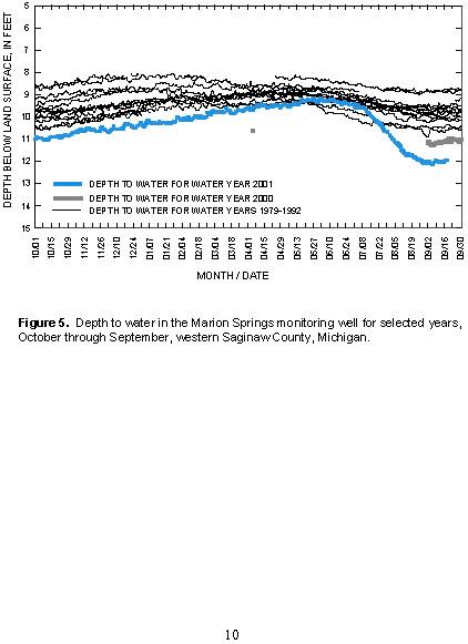
During the USGS study, water levels were measured in two monitoring wells in western Saginaw County. Marion Springs monitoring well (fig. 1) was selected to monitor background conditions (assumed to not be influenced by irrigation pumping). The second monitoring well (USGS MW; fig. 1) was chosen to measure expected influences of irrigation wells.
The assumed background well is a USGS monitoring well (station number 431457084194401; Blumer and others, 1991) near Marion Springs, Michigan (fig. 1). This well is completed in the Saginaw aquifer. Water-level records from 1979 through 1991 show the well was unaffected by irrigation (fig. 5). Continuous monitoring of this well ceased in December 1991, but was resumed in September 2000 as part of this study. Water-level changes in this well were expected to reflect regional climate responses to factors that control recharge and discharge (seasonal/long-term changes of rainfall, evapotranspiration rates, and so on). However, inspection of the water-level record for the Marion Springs well (fig. 6) shows a sharp water-level decline related to the onset of the irrigation season in July, 2001. Water levels continued to decline through the irrigation season and had declined by about 3 ft at the end of the season (fig. 5). This 3-ft decline of water level is most likely caused by irrigation at a well 4.5 mi northeast of the Marion Springs well. The USGS learned from local irrigators that a large-capacity irrigation well was installed and operated in 1999 at a farm about 4.5 mi north of the Marion Springs monitoring well (fig.1). This newly installed irrigation well also is completed in the Saginaw aquifer, providing further evidence that the sharp drop in water level is related to irrigation pumping.
Water levels were also monitored at USGS MW (station number 432206084194801; established 2000) located about 0.5 mi from irrigation well IR-4 in Lakefield Township (fig. 1). A water-level recorder was installed in this well by the USGS in September 2000. The water level at USGS MW was about 6.5 ft below land surface prior to the onset of irrigation (fig. 7). The water-level data show that irrigation pumping lowered water levels by about 20 ft. During August 2001, the relatively stable fluctuation of drawdown and recovery (between 21 and 25 ft below land surface) is a function of controlled pumpage by the farm near the monitoring well; the irrigator used real-time data available on the Internet to reduce irrigation withdrawals when water-level declines approached 25 ft below land surface (Grant Cooper, LDS, oral commun., 2001). This controlled irrigation procedure resulted in a new pumping cycle consisting of 12 hours of pumping and 2 to 2.5 days of recovery before the next pumping cycle (fig. 7). The missing data on figure 7 (June 29-July 3, 2001) was due to installation of real-time telemetry so water-level measurements could be accessed through the Internet.
DEVELOPMENT OF NUMERICAL MODELS
The potential drawdown effects of irrigation pumpage were simulated by
developing flow models of the glaciofluvial and Saginaw aquifers. The generalized
models assume radial, axisymmetric two-dimensional ground-water flow toward
irrigation wells. Models also assume that aquifers are homogenous and isotropic.
This approach was taken because the limited amount of hydrogeologic data available
did not allow more complex regional models. In addition, this approach offers
the relative ease of formulating a simulation, making it easy to estimate drawdown
at any distance.
Several investigators (Rutledge, 1991; Reilly and Harbaugh, 1993; Johnson and others, 2001) have developed axisymmetric-flow models for aquifer-test analysis. These axisymmetric-flow models have proven to be reliable and effective tools in simulating ground-water-flow conditions caused by production wells. For this study, ground-water-flow simulations were developed using RADMOD (Reilly and Harbaugh, 1993), which is a preprocessor to MODFLOW (McDonald and Harbaugh, 1988), the USGS modular finite-difference ground-water-flow model. A description of RADMOD and its applications can be found in Reilly and Harbaugh (1993). The RADMOD preprocessor is used to develop a generalized finite-difference (GFD) package (Harbaugh, 1992). The GFD package provides input to MODFLOW.
Four different simulations were formulated to represent the hydrologic variability of the aquifer system studied. One simulation was developed to model the Saginaw aquifer. Because there is an order of magnitude difference in the hydraulic conductivity of the glaciofluvial aquifer (Soils and Materials Engineers, written commun., 2001), three additional simulations were developed to model a range of possible water-level declines in response to irrigation pumping. In contrast, the Saginaw aquifer is relatively homogenous and laterally continuous, therefore one simulation was considered adequate to demonstrate the effects of irrigation pumping. Although all simulations are hypothetical, they are based on the analysis of actual aquifer tests.
Discretization
A series of discrete cells (a grid) is formulated to represent the actual physical system modeled. The RADMOD preprocessor creates a model grid using cylindrical coordinates. Conceptually, the model can be considered a series of concentric-cylindrical shells. The first shell r1 is located at the radius of the well. For this study, models used 100 cylindrical shells extending a distance of approximately 10 mi radially from the center shell. Each shell is expanded outward away from a well using the relation:
![]()
where ri (ft) is the radius interior to ri+1, a is the geometric expansion factor, and ri+1 (ft) is the radius of the shell following ri (Reilly and Harbaugh, 1993). An example model grid is illustrated in figure 8. Grid shells are closely spaced at the center of models. The fine discretization of grid nodes was necessary to accurately model steep-head gradients that are produced by the large volume of pumping associated with irrigation wells. Because head gradients are not as steep farther away from pumping wells, shell spacing was increased away from wells.
Vertical discretization of the model was developed primarily on information from geologic logs. Some wells also have geophysical logs available, which were used to assist in the delineation of model layers. The layers chosen to represent aquifers and confining units are shown in table 2. For the Saginaw aquifer system, the 4 upper layers represent the confining unit, and the lower 5 layers represent the alternating sandstone (aquifer) and shale (confining) units. In the glaciofluvial simulations, the upper 2 to 3 layers represent the confining units, and the lower layers represent the aquifer material (table 2).
Hydraulic properties and boundary conditions
Hydraulic properties were initially assigned to layers based on data from aquifer tests or from values listed in the literature (Freeze and Cherry, 1979). The final calibrated hydraulic properties assigned to model layers are summarized in table 2.
|
[ft, feet; ft/d, feet per day. Note: very small numbers are expressed in scientific notation for compactness, where the value is multiplied by a power of 10, and the value following “E” is the exponent. For example, 1.0E-07 would be 1*10-7 or 0.0000001] | |||||
|
Simulation |
Layer |
Thickness (ft) |
Hydraulic conductivity (ft/d) |
Vertical hydraulic conductivity (ft/d) |
Storage coefficient |
|---|---|---|---|---|---|
|
Saginaw |
1 |
120 |
1.0E-07 |
1.0E-07 |
1.0E-04 |
|
2 |
20 |
0.010 |
1.0E-03 |
1.0E-03 |
|
|
3 |
35 |
1.0E-07 |
1.0E-07 |
1.0E-04 |
|
|
4 |
35 |
1.0E-08 |
1.0E-08 |
1.0E-06 |
|
|
5 |
125 |
5.8 |
0.63 |
1.2E-06 |
|
|
6 |
10 |
1.0E-07 |
1.0E-08 |
1.0E-06 |
|
|
7 |
125 |
5.8 |
0.63 |
1.2E-06 |
|
|
8 |
30 |
1.0E-07 |
1.0E-08 |
1.0E-06 |
|
|
9 |
55 |
5.8 |
0.63 |
1.2E-06 |
|
|
Glaciofluvial 1 |
|||||
|
1 |
7 |
0.010 |
1.0E-03 |
1.0E-03 |
|
|
2 |
45 |
1.0E-08 |
1.0E-09 |
1.0E-06 |
|
|
3 |
48 |
10 |
1.0E-03 |
6.0E-06 |
|
|
4 |
25 |
9.9 |
0.006 |
1.6E-06 |
|
|
5 |
60 |
20 |
0.011 |
1.9E-05 |
|
|
Glaciofluvial 2 |
|||||
|
1 |
6 |
0.010 |
1.0E-03 |
1.0E-03 |
|
|
2 |
79 |
1.0E-08 |
1.0E-09 |
1.0E-06 |
|
|
3 |
60 |
20 |
2.6 |
4.0E-06 |
|
|
4 |
13 |
1.0E-08 |
1.0E-09 |
1.0E-06 |
|
|
5 |
15 |
20 |
2.6 |
4.0E-06 |
|
|
6 |
14 |
1.0E-08 |
1.0E-09 |
1.0E-06 |
|
|
7 |
10 |
20 |
2.6 |
4.0E-06 |
|
|
Glaciofluvial 3 |
|||||
|
1 |
6 |
1.0E-03 |
1.0E-04 |
1.0E-03 |
|
|
2 |
74 |
1.0E-08 |
1.0E-09 |
1.0E-06 |
|
|
3 |
50 |
1.0E-03 |
1.0E-04 |
1.0E-04 |
|
|
4 |
65 |
140 |
13 |
6.6E-06 |
|
|
5 |
29 |
1.0E-06 |
1.0E-07 |
1.0E-06 |
|
|
6 |
42 |
10 |
1.0E-01 |
1.0E-04 |
|
|
7 |
6 |
5.8 |
0.5 |
1.5E-06 |
|
Delineation of hydrologic boundaries, or how water enters and leaves an aquifer system is a key step in any modeling exercise. For the scenarios simulated in this study, a specified-head boundary was defined at the outer edge of models. Model boundaries were set approximately 10 mi away from pumping wells. This 10-mi specified-head boundary was assumed to be an appropriate outer boundary for the aquifer system, based on inspection of water-level records of a USGS monitoring well in Marion Springs (fig. 1 and fig. 5). For the period of record (1979-91), the USGS Marion Springs monitoring well showed no indication of water-level change that could be attributed to irrigation pumping. A no-flow boundary also is assumed for the base of all model simulations. Initial head conditions for all models were based on water levels measured in irrigation and monitoring wells. The water level measured in irrigation wells prior to aquifer testing was used as the initial head value.
In some cases, simulated irrigation wells were open to several model layers
in an attempt to represent complexities of the aquifer system. RADMOD requires
the pumping rate to be divided among these layers. To model pumping rates,
a conductivity-flux-weighted average was estimated for each layer by means of
the following relation: 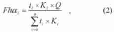
where Fluxl (ft3/d) is the amount of water pumped from layer l, tl (ft) is the thickness of the target (producing) layer, Kl (ft/d) is the hydraulic conductivity of the target layer, Q (ft3/d) is the pumping rate, ti (ft) is the thickness of a layer affected by pumping, Ki (ft/d) is the hydraulic conductivity of a layer affected by pumping, x is the first layer affected by pumping, and n is the last layer affected by pumping.
Model calibration
Transient-model simulations were calibrated to aquifer tests performed on irrigation wells (Soils and Materials Engineers, written commun., 2001). For each irrigation well, the pumping stress and duration of the corresponding aquifer test was simulated. The observed drawdown in observation or pumping wells for each 24-hour aquifer test was used as the calibration target for the simulations(table 3). In each simulation, the irrigation well was not pumped for a specified time period and was then pumped for a period of 24 hrs. For model calibration, the simulated water levels after 24 hrs were compared to measured water levels. In all cases, hydraulic conductivity and storage coefficients were adjusted within physically reasonable limits so that simulated drawdowns matched observed drawdowns from the aquifer tests. In one case, hydraulic conductivity was increased by as much as 40 ft/d from the initial estimate. For all scenarios, storage coefficients were decreased by at least an order of magnitude from initial estimates. The largest acceptable deviation of a simulated drawdown value from an observed drawdown was 1.5 ft. After a simulation met this criterion, the simulation was considered calibrated (table 3). Calibrated models were then used to simulate water-level declines related to irrigation, using a 3-month irrigation season.
Assumptions and limitations
Uncertainty is inherent in any simulated water-level response to pumping.
For the simulations described in this report, the aquifer system modeled is
assumed to be homogenous and isotropic. Although the aquifer system is neither
homogenous nor isotropic, the available hydrologic data do not allow inclusion
of heterogeneities or other complexities to simulate effects of irrigation.
Therefore, models provide only estimates of aquifer response to irrigation pumping.
Despite simulating three different cases in the glaciofluvial aquifer, the simulations do not represent the entire range of aquifer properties of glaciofluvial aquifers in the study area, because of the inherent heterogeneous nature of glacial deposits. Rather, the three simulations provide the best estimate of water-level declines based on available data.
Recharge is not applied to the model because the location and amount of recharge is uncertain; recharge is also unlikely to occur through the thick clay-rich beds that overlie the aquifer system. There is also uncertainty of pumping rates and duration of pumping of irrigation wells. Irrigation wells not operating at optimum efficiency are pumping less water than the volumes predicted during aquifer tests. Another limitation of the axisymmetric-flow models is that a regional ground-water gradient cannot be applied. This is a minor concern in the study area because the magnitude of the ground-water gradient is very small in relation to gradients caused by irrigation pumping.
Simulation results
Several simulations were performed to determine effects of irrigation on water levels. Over a 3-month pumping cycle, numerical simulations of water-level decline in 4 irrigation wells show a predicted range of drawdowns to be 5.3 to 20 ft at 0.5 mi, and 1.7 to 6.9 ft at 3 mi from irrigation wells. At a distance of about 4.5 mi from an irrigation well, water levels in the Saginaw aquifer would be expected to decline by about 3 ft. This simulation is in close agreement with the observed decline at the USGS monitoring well in Marion Springs during the 2001 irrigation season (fig. 6). Model results are summarized in table 4.
The calibrated model for the Saginaw aquifer was used to simulate water-level changes for USGS MW. Results from this simulation (fig. 9) show excellent agreement with measured USGS MW water levels (fig. 7). As mentioned previously, the water level in USGS MW (near the irrigation well in the Saginaw aquifer) was about 6.5 ft below land surface before the onset of irrigation (fig. 7). USGS MW data show that irrigation pumping lowered water levels by more than 20 ft during the agricultural season (June-Sept., 2001). A simulation of the Saginaw aquifer also indicates a water-level decline of 20 ft from the prepumping water level. Inspection of the early data (prior to July 21, 2001; fig. 7) indicates a cycle of 12 hours from peak to trough of the water-level records, which agrees well with the pumping cycle assumed for the simulations.
Although the simulated water levels for the Saginaw aquifer closely match the measured water levels in USGS MW (fig. 9), a somewhat smaller amplitude of fluctuation in water levels between pumping cycles is simulated, compared to observed water levels at USGS MW (fig. 7). At 0.5 mi from irrigation well IR-4, fluctuation related to one 12-hr pumping cycle is about 2 ft (fig. 7). The model simulates 1.2 ft of fluctuation as a result of the same pumping scenario (fig. 9). Data from the USGS MW (fig. 7) suggest that water levels in the aquifer would have continued to decline below 26.5 ft if the 12-hr pumping cycle had been continued. Because the farm altered the pumping cycle at drawdowns of about 25 ft below land surface, water levels appear to reach a steady-state. The apparent steady-state would probably not be achieved if the 12-hr pumping cycle was used for the entire irrigation season, and would likely lead to water-level declines substantially more than 25 ft below land surface.
Effects of Ground-water withdrawals for irrigation on Residential Wells
Analysis of available data indicate that large volumes of water pumped
for irrigation resulted in drawdown that causes substantial water-level declines
in nearby residential wells. Because the glaciofluvial and the Saginaw aquifers
are separated by a shale confining unit in most of the study area, residential
wells will be affected by irrigation wells that tap the same aquifer.
This is one explanation why one residential well may fail to pump water while a nearby residential well, which taps a different aquifer, may not fail to pump water.
The use of jet-type pumps in residential wells also can be a factor in loss of or reduced well yield. Many residential wells in the study area are 2 inches in diameter and equipped with shallow jet pumps. Shallow jet pumps can pump water only if water is within about 20 ft of land surface. Given a preirrigation water level of approximately 6 to 7 ft below land surface, an irrigation induced water-level decline of approximately 14 ft would cause well failure or reduction of flow. On the basis of observed data and modeling results, a 14 ft or greater water-level decline can occur up to 1.1 mi (depending on the aquifer) from large-volume irrigation wells, causing shallow jet pumps near such wells to fail to pump water (fig. 10). A submersible pump set deep in a similar well, however, would still produce water because it operates by a different mechanism.
Seasonal fluctuations typically result in about 3 ft of water-level decline during the summer, as described in the “Hydrogeologic Setting” section of this report. Combining a 3-ft seasonal decline with a preirrigation water level of 6.5 ft below land surface, irrigation-related water-level declines of as little as 11 ft would likely result in well failure of a shallow jet pump during the summer. Figure 10 illustrates simulated relations between distance from irrigation wells and the related drawdowns. In cases of below-average precipitation and recharge, even less drawdown from irrigation wells would likely affect residential wells equipped with shallow jet pumps. A list of other problems that may also lead to failure of a well to meet residential needs is provided in table 5.
SUGGESTIONS FOR FUTURE STUDY
The study described in this report provides information on relations of water-level declines to pumping of irrigation wells in western Saginaw County. Interpretations and predictions beyond those presented herein, are not possible to make without more detailed hydrologic data. Additional studies would greatly enhance the ability to describe and model hydrogeology and ground-water-level responses to water use in this area and would facilitate long-term water management, including the following:
· Long-term water-level monitoring of multiple wells in the glaciofluvial and Saginaw aquifers in order to differentiate between human imposed effects and natural effects on water levels.
· Development of a regional model to accurately predict effects of multiple irrigation wells pumping throughout the region, allowing for best management of water resources in the area.
a. Studies to refine aquifer boundaries and aquifer properties.
b. Studies of recharge processes/areas, evapotranspiration, and other components of the sub-regional water budget.
c. Age-dating of ground water by use of chlorofluorocarbons and radionuclides to better understand recharge rates.
Summary and Conclusions
Distance-drawdown predictions modeled by use of hydrogeologic data from
irrigation wells indicate water-level declines as much as 12 feet at distances
of 1.5 miles from large-capacity wells, due solely to pumping for irrigation.
At a distance of 0.5 miles from irrigation wells, conservative models predict
as much as 20 feet of drawdown.
Given a preirrigation water level of 6.5 feet, residential wells equipped with shallow jet pumps would likely fail to pump water under conditions of about 14 feet of water-level decline where the residential and irrigation wells tap the same aquifer. When seasonal water-level declines are considered, shallow jet pumps in wells as far as 1.5 miles away from irrigation wells also may fail to pump water.
On the basis of monitoring well data and simulations of drawdown as a function of distance from irrigation wells, large ground-water withdrawals for irrigation are substantially reducing nearby water levels. Residential-well failure during the irrigation season, however, does not mean that loss or reduced well yield is entirely the result of irrigation pumping. There are many variables that contribute to the loss or reduction of well yield, such as aquifer characteristics, recharge rates, well construction, pump type, pump condition, and other related variables. Each of these variables needs to be evaluated on a well-by-well basis.
Publication
Hoard, C.J. and Westjohn, D.B., 2001, Simulated
Effects of Pumping Irrigation Wells on Ground-Water Levels in Western Saginaw
County, Michigan: U.S. Geological Survey Water Resources Investigations Report
01-4227.
In cooperation with the Michigan Department of Environmental Quality
Baltusis, M.A., Quigley, M.F., and Mandle, R.J., 1992, Municipal ground-water development and withdrawals in the central Lower Peninsula of Michigan, 1870-1987: U.S. Geological Survey Open-File Report 91-215, 89 p.
Barton, G.J., Mandle, R.J., and Baltusis, M.A., 1996, Predevelopment freshwater heads of the glaciofluvial, Saginaw, and Marshall aquifers in the Michigan Basin: U.S. Geological Survey Open-File Report 95-319, 15 p.
Blumer, S.P., Larson, W.W., Minnerick, R.J., Whited, C.R., and LeuVoy, R.L., 1991, Water resources data Michigan, water year 1991: U.S. Geological Survey Water-Data Report MI-91-1, 284 p.
Farrand, W.R., and Bell, D.L., 1982, Quaternary geology of southern Michigan: Ann Arbor, Michigan, Department of Geological Sciences, University of Michigan, scale 1:500,000.
Freeze, R.A., and Cherry J.A., 1979, Groundwater: Englewood Cliffs, N.J., Prentice-Hall Inc., 604 p.
Harbaugh, A.W., 1992, A generalized finite-difference formulation for the U.S. Geological Survey modular three-dimensional finite-difference ground-water flow model: U.S. Geological Survey Open File Report 91-494, 60 p.
Holtschlag, D.J., 1996, A generalized estimate of ground-water recharge rates in the Lower Peninsula of Michigan: U.S. Geological Survey Water-Supply Paper 2437, 37 p.
Johnson, G.S., Cosgrove, D.M., and Frederick, D.M., 2001, A numerical model and spreadsheet interface for pumping test analysis: Ground Water, v. 39, no. 4, p. 582-592.
Martin, H.M., comp., 1955, Map of the surface formations of the southern Peninsula of Michigan: Michigan Geological Survey Publication 49, scale 1:500,000.
McDonald, M.G., and Harbaugh, A.W., 1988, A modular three-dimensional finite-difference ground-water flow model: U.S. Geological Survey, Techniques of Water-Resources Investigations, book 6, chapt. A1, 586 p.
Meissner, B.D., Long, D.T., and Lee, R.W., 1996, Selected geochemical characteristics of ground water from the Saginaw aquifer in the Michigan Basin: U.S. Geological Survey Water-Resources Investigations Report 93-4220, 29 p.
Reilly, T.E., and Harbaugh, A.W., 1993, Simulation of cylindrical flow to a well using the U.S. Geological Survey modular finite-difference ground-water flow model: Ground Water v. 31, no. 3, p. 489-494.
Rutledge, A.T., 1991,
An axisymmetric finite-difference flow model to simulate drawdown in and around
a pumped well: U.S. Geological Survey, Water-Resources Investigations Report
90-4098,
33 p.
Westjohn,
D.B., and Weaver, T.L.,
1996, Configuration of freshwater/saline-water interface and geologic controls
of distribution of freshwater in a regional aquifer system, central Lower Peninsula
of Michigan: U.S. Geological Survey, Water-Resources Investigations Report
94-4242, 44 p.
Westjohn, D.B., and Weaver, T.L., 1998, Hydrogeologic framework of the Michigan Basin regional aquifer system: U.S. Geological Survey Professional Paper 1418, 47 p.