
Water Resources of Michigan
Ground-Water Quality Atlas of Oakland County, Michigan
US Geological Survey Water-Resources Investigation 00-4120
Lansing, Michigan August 2000
Table of Contents including Figures, Maps, Graphs, Tables, Appendix, Conversion
Factors and Vertical Datum, and Additional Information.
http://mi.water.usgs.gov/pubs/WRIR/WRIR01-4120/WRIR00-4120TOC.php
ABSTRACT
The U.S. Geological Survey (USGS), in cooperation with Oakland County Health
Division (OCHD), collected 140 water samples from 38 wells in Oakland County
during 1998 to better understand ground-water quality. OCHD had observed temporal
variations in concentrations of various constituents, so two additional sets
of samples were collected to evaluate potential short-term variability related
to sample collection procedures and long-term seasonal variability. Replicate
samples from 28 wells were analyzed in the Michigan Department of Environmental
Quality (MDEQ) Drinking Water Laboratory to compare MDEQ's analytical results
to those obtained from the USGS National Water Quality Laboratory. Several additional
databases describing population, land use, water supply, soils, geology, and
flows of ground water and surface water are presented in the first part of the
report to assist in interpreting the water-quality data. Maps created from these
databases are provided in the first portion of the report as an extension of
the study-area description.
The U.S. Environmental Protection Agency (USEPA) has established Maximum Contaminant Levels (MCL) and Secondary Maximum Contaminant Levels (SMCL) for which samples were analyzed in this study. Water from the 38 wells sampled by the USGS did not exceed the SMCL or MCL for sulfate, fluoride, or nitrite. However, water from 26 wells exceeded the SMCL for iron, water from 12 wells exceeded the SMCL for manganese, and water from 12 wells exceeded the SMCL for dissolved solids. Water from two wells exceeded the MCL for nitrate, although nitrate concentrations in water from most wells was below the detection limit. Water from seven wells exceeded the SMCL for chloride, and water from all wells contained detectable concentrations of chloride. Water from five wells exceeded the MCL for arsenic, and most of the wells sampled contained detectable concentrations of arsenic. These five wells were identified from previous MDEQ analyses to have elevated arsenic concentrations, and were sampled to obtain additional chemistry information. Replicate samples were collected from 26 of the 38 wells for analysis at the MDEQ Drinking-Water Laboratory to compare the results with the USGS National Water Quality Laboratory. The results of the replicate analyses indicate close agreement between the laboratories, with mean differences for nitrate, chloride, and arsenic of 0.10 milligrams per liter (mg/L) as nitrogen, 6.8 mg/L, and 0.0008 mg/L, respectively between the USGS and MDEQ analyses. Potential health effects associated with ingesting nitrate, chloride, and arsenic are provided with the water-quality data, along with references for further information.
Introduction
In 1996, the U.S. Geological Survey (USGS), in cooperation with the Michigan
Department of Environmental Quality (MDEQ), the University of Michigan, and
nine counties in southeastern Michigan, began a study of the occurrence and distribution of arsenic in ground water in southeastern
Michigan. The early results of this study raised broader concerns in Oakland
County about the quality of ground water used for drinking water. In response
to these concerns, the USGS, in cooperation with the Oakland County Health Division
(OCHD) initiated a study of distributions of arsenic, nitrate, and chloride
in ground water in Oakland County. A series of USGS Fact Sheets were produced
in December 1998 to present maps and information to residents of Oakland County
about the distribution and potential health effects of these chemicals in ground
water.
Understanding the distribution of these chemicals required the compilation of several supporting data sets describing the geologic and hydrologic setting of Oakland County. These data sets are presented in the first part of this report. Water samples from 38 wells across Oakland County were analyzed for arsenic, nitrate, chloride, and more than 20 additional physical and chemical characteristics. Complete analytical results are provided in Appendix 1. A comparison of analytical results from the USGS National Water-Quality Laboratory (NWQL) and the MDEQ Drinking Water Laboratory is presented in Appendix 2.
Purpose and Scope
This report provides information on the distribution of arsenic, nitrate and
chloride in ground water in Oakland County and the potential health effects
of each chemical. Analytical results are presented for water samples collected
by the USGS in Oakland County in 1998, as well as several supporting spatial
databases describing the demographic, geologic, and hydrologic context of Oakland
County. This report also provides several maps, generated by the Center for
Applied Environmental Research at the University of Michigan-Flint (CAER) from information in MDEQ databases, to describe the occurrence
of arsenic, nitrate, and chloride in ground water.
Acknowledgments
The author gratefully acknowledges the assistance of Dr. Thomas Gordon, Robert
Long, and Karen Kubik of Oakland County Health and Human Services in obtaining
historical data, coordinating access to sample sites, and providing background
information for interpreting the water-quality data. Scott Oppmann and Brian
Ely of the Oakland County GIS Utility provided digital base map data with municipal
boundaries. Dr. Richard Hill-Rowley and Matt Malone of CAER provided assistance
with validating and geocoding the MDEQ database, as well as with strategies
for mapping the data at the county scale. Thomas McClain of the CAER mapped
the elevation of the water-table surface.
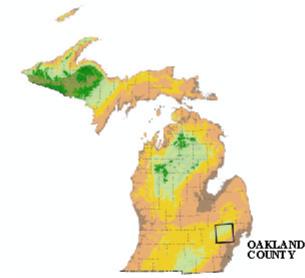
OAKLAND COUNTY, MICHIGAN
A variety of spatial databases were generated or modified for use in this study, and are presented in the next several pages to provide a context for the study. Included are descriptions of the glacial geology, soils, surface- and ground-water resources, as well as summary information about water-use, population growth, and land-use change in Oakland County. Oakland County, with a land area of 900 square miles, contains 25 survey townships and is the largest county in the Lower Peninsula of Michigan. With more than 1.2 million residents, Oakland County is the second most populous county in Michigan.
Population Growth and Land-Use Change
Oakland County has grown dramatically in the last several decades. The Southeast
Michigan Council of Governments (SEMCOG) provides estimates of actual population
based on information from county and local governments to supplement Census
data. The population has increased from about 700,000 in 1960 to nearly 1.2
million in 1998. The rate of population growth has been relatively consistent,
with the population increasing by more than 100,000 people per decade. Population
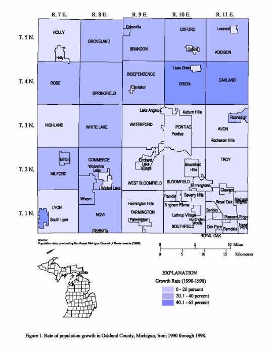
growth has not been spatially uniform (fig. 1). Population growth between 1990
and 1998 has exceeded 60 percent in some municipalities, and has exceeded 20
percent in 18 of 58 minor civil divisions (Southeast Michigan Council of Governments,
1999).
The expansion of residential areas resulting from the increase in population has resulted in marked changes in land use. A comparison of land-use data compiled by the Michigan Department of Natural Resources (1978) and SEMCOG data compiled in 1995 indicates an increase in urban land use, primarily residential, accompanied by decreases in agricultural land, pasture land, and forest land (table 1). While some of these differences may be because of differences in the methods of compilation between agencies (specifically identification of wetlands in the 'Other' category), the trend is toward increasing allocation of land for urban use, with decreasing allocation for agriculture, forest, and pasture.
Table 1. Land use in Oakland County as a percentage of total county area, 1978 and 1995
|
Land use
|
1995
|
1978
|
|---|---|---|
|
(percent)
|
(percent)
|
|
|
Urban
|
48.7 | 39.3 |
|
Agriculture
|
11.7 | 15.0 |
|
Pasture
|
16.2 | 21.3 |
|
Forest
|
8.4 | 13.7 |
|
Other
|
15.0 | 10.7 |
The effects of human activities on water resources, whether ground water or surface water, are complex (Winter and others, 1998). The increased proportion of the county devoted to urban and residential land uses is accompanied by more wells that extract water, more impervious surfaces that block or redirect recharge, and more storm drains that divert precipitation into streams instead of aquifers. Over time, this can alter the availability and quality of hydrologic resources, both ground water and surface water, in Oakland County. Modifications in land use may also affect the proportions of ground water and surface runoff in rivers and streams, which can affect the chemistry, temperature, and general quality of the water for wildlife and for recreation. The need to better understand how the increased use of water for agriculture, recreation, and residential household uses affects ground-water and surface-water resources will surely increase as development intensifies (Winter and others, 1998).
Figure 1. Rate of population growth in Oakland County, Michigan, from 1990 through 1998.
Water Supply
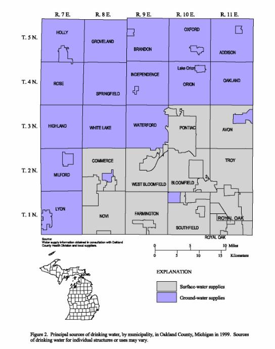
Most of Oakland County is served by public water supplies. These supplies are
subject to regulation by Federal, State, and other authorities to ensure the
water produced meets public health standards. The Detroit Water and Sewerage
Department (DWSD) provides 137 million gallons per day (MGD) of water to the
southeastern townships of Avon (Rochester Hills), Pontiac, Troy, Bloomfield,
West Bloomfield, Royal Oak, Southfield, Farmington, Novi and Commerce (fig.
2). Several additional mains have been constructed to provide water to adjoining
areas. Water provided by DWSD is drawn from Lake Huron and Lake St. Clair, as
well as the St. Clair River and Detroit River.
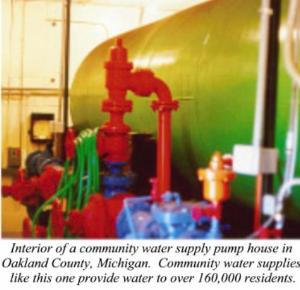
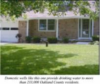
More than 140 smaller community supplies use ground-water resources to provide 21.4 MGD to more than 160,000 residents (C. Luukkonen, USGS, written commun., 1999). The communities served by these supplies range in size from Waterford Township, with a population of more than 70,000 (Southeast Michigan Council of Governments, 1999), to individual subdivisions, with only a few homes. More than 233,000 Oakland County residents are not connected to public water supplies, but obtain water from domestic wells. These withdrawals amount to approximately 16.7 MGD (C. Luukkonen, USGS, written commun., 1999). Domestic wells are not currently monitored by any governmental agency, and are the responsibility of the owner.
Surface-Water Resources
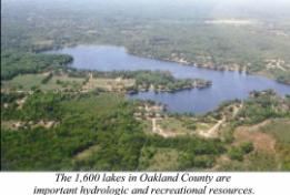
Surface-water resources abound in Oakland County. More than 1,600 lakes of varying
sizes were recorded in a 1958 inventory (Humphrys, 1962). A substantial number
of these lakes are large enough for recreational use, such as boating, swimming,
and fishing. Most of these lakes receive water from ground water most of the
year (Mozola, 1954).
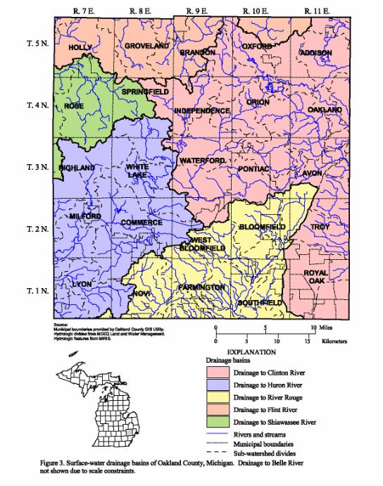
Oakland County spans the headwaters of six major rivers (fig. 3). The Shiawassee and Flint Rivers drain the northwestern part of the County, eventually joining the Saginaw River to flow into Lake Huron. The Huron River drains the southwestern part of the county, delivering the water to Lake Erie. The Clinton River in the north and the River Rouge in the south drain the central and southeastern parts of the county into Lake St. Clair and the Detroit River. The Belle River drains a very small area (less than 1 sq. mi.) of Addison Township. More than half of the water flowing in these rivers over the course of a year is ground-water discharge to the river through the streambed (Holtschlag and Nicholas, 1998).
Surficial Geology
Nearly all of the hills and lakes in Oakland County were formed during the retreat
of the last continental glacier, approximately 14,000 years ago (Winters and
others, 1985). For the preceding 60,000 years, the area that is now Oakland
County was intermittently covered by as much as a mile of ice. During the retreat
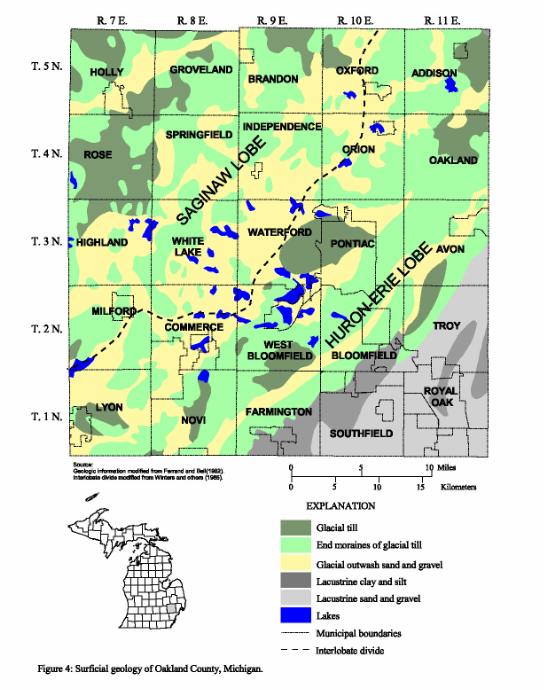
of the ice, an ice-free area formed between the Saginaw Lobe in the northern
part of the county and the Huron-Erie Lobe to the south (fig. 4), the axis of
which tracks through Commerce, Waterford, and Oxford (Leverett and Taylor, 1915;
Winters and others, 1985). This area formed a conduit for large quantities of
water and sediment flowing off the melting glacier, known as outwash. Outwash
environments deposit sorted sediments, so that materials of a certain size and
composition are layered vertically and are exposed together on the landscape.
A broad outwash plain (shown in yellow in figure 4) stretches across central
Oakland County from northeast to southwest.
On either edge of the outwash plain region are areas of moraine and other types of till (shown in green hues in figure 4), deposited directly by the ice at the margins of the glacial lobes. The materials in these features are unsorted, and include clays, sands, pebbles, and boulders. These areas usually have much higher clay fractions than the outwash plain region, which results in lower permeability.
Following the retreat of the ice back to the Great Lakes basins, large lakes formed from meltwater occurred at much higher elevations than the current elevations of the Great Lakes (Eschman and Karrow, 1985). The beds of these lakes collected clays and other sediments in broad blankets. The highest of these lakes in the Huron-Erie basin was Lake Maumee, which maintained an elevation between 775 and 810 ft above sea level (covering much of southeastern Oakland County) for a period of approximately 300 years starting 14,000 years ago (Eschman and Karrow, 1985). The beds of these proglacial lakes are evident in the flat-lying, clay-rich sediments of southeastern Oakland County (shown in gray tones in figure 4). These clay-rich sediments have dramatically lower permeability than the outwash sediments.
The thickness of these glacial materials vary greatly across the county. The thickness of the surficial sediments exceeds 400 feet across the central part of the county, but can be less than 100 feet in the southeast and northwest corners (Twenter and Knutilla, 1972). Throughout most of the county, the surficial deposits are the primary aquifer. Fewer than 3 percent of the wells in the county's WELLKEY database are completed in bedrock.
The underlying bedrock units throughout most of the county are not considered good sources of potable water, and water drawn from these units is frequently high in sulfate, iron, chloride, and dissolved solids. The Marshall Sandstone is a productive bedrock aquifer for the northwestern townships of Holly, Groveland, Brandon, and Rose. Even in this area, the vast majority of wells are completed in the glacial sediments.
Figure 4. Surficial geology of Oakland County, Michigan.
Soils
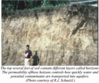
The soils of Oakland County are the direct result of the surficial geologic
processes previously described. Physical and chemical characteristics reported
by the Soil Conservation Service (1982) show patterns similar to the surficial
geology map shown previously.
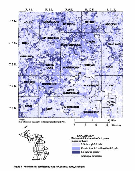
Minimum soil permeability, for example, ranges over two orders of magnitude, from 0.06 inches/hour (in/hr) to 20 in/hr. The region with minimum infiltration rates of 6 in/hr or greater closely resembles the region mapped as outwash (fig. 5). Infiltration rates directly affect the amount of recharge, and thus the potential for transport of contaminants into an aquifer. The lowest permeability soils correspond spatially to till and lake-bed sediments. High permeability, sandy soils have been widely identified as being susceptible to contamination by anthropogenic pollutants, such as nitrate (Kittleson, 1987; Fetter, 1994).
The chemical properties of the soils also reflect the surficial geologic processes. The highest concentrations of calcium carbonate in the soil are generally clustered in regions formed of till. Calcium carbonate concentrations are generally lower in the outwash plain region located in the central part of the county. Bicarbonate (HCO3-), an ion formed when calcium carbonate is dissolved by infiltrating water, has been shown to encourage the dissolution of arsenic (Kim, 1999).
Figure 5. Minimum soil permeability rates in Oakland County, Michigan.
Ground-Water Resources
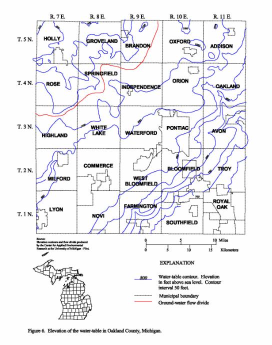
The CAER developed a map of ground-water levels in Oakland County (fig. 6),
derived from the elevations of rivers and lakes and the elevations of ground
water in the glacial aquifer. Ground-water elevations were obtained from drillers'
logs and Oakland County's WELLKEY database. Because the drillers' logs were
collected over a period of several decades, the derived surface represents an
approximation over time, rather than a specific time.
In general, the configuration of the water table is a subdued version of the landscape topography. Accordingly, the water-level map developed by the CAER shows a region of higher water levels along the northern edge of the outwash plain region, corresponding to the part of Oakland County where the land surface is highest. The high region in the water table surface forms a ground-water-flow divide. Northwest of this divide, ground water generally flows towards Saginaw Bay. Southeast of this divide, ground water generally flows toward Lake Erie and Lake St. Clair.
This map represents the water levels in the glacial aquifer only. Evaluation of Oakland County's WELLKEY database indicates more than 97 percent (8,458 of 8,654) of the wells in the database are completed in the glacial aquifer. Several examples of confined aquifers and artesian wells have been noted by authors in the past (Mozola, 1954; Leverett and others, 1906). In these regions, water within these confined systems may be under pressure, and would rise to a different level than the level portrayed in figure 6.
Figure 6. Elevation of the water-table surface in Oakland County, Michigan.
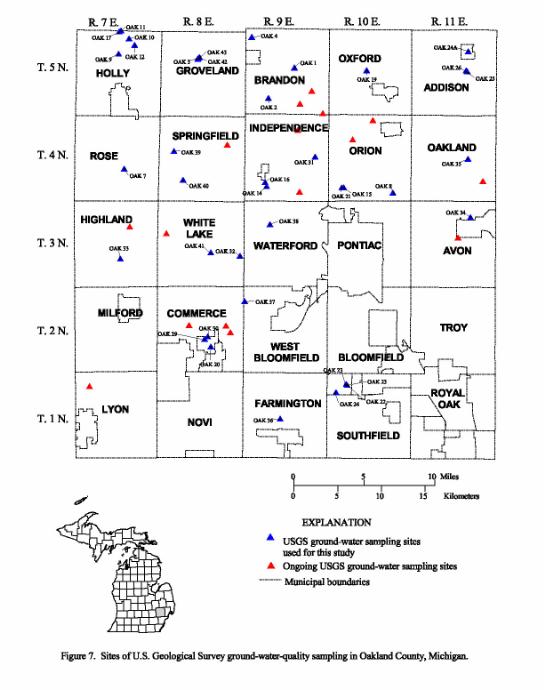
Sites of USGS Ground-Water-Quality Sampling
The USGS collected water samples from 68 wells in Oakland County in 1997 and
1998 (fig 7). Thirty of these wells were sampled as part of ongoing USGS activities.
The results of these analyses are presented in Blumer and others (1998).
Thirty-eight wells were sampled specifically for this project between June and December 1998. These wells were selected for several reasons. All selected wells had a previous water quality analysis in the Michigan Department of Environmental Quality (MDEQ) database. The water from approximately half of these wells had exceeded at least one U.S. Environmental Protection Agency (USEPA) Maximum Contaminant Level (MCL) or Secondary MCL (SMCL) on at least one occasion. Additional wells with previous water chemistry information and lower concentrations of the chemical constituents of concern were selected in the vicinity of the wells with exceedances of the regulatory contaminant levels.
All but six of the wells selected for sampling were privately owned domestic water wells supplying a single-family dwelling. Two of the selected wells supplied water to institutions, one to a restaurant, one to a car wash, one to a community water supply, and one to a government building. Well depths, obtained from well construction logs when available, are included in appendix table 1C.
Two additional sets of samples were collected in December 1998. Each set included samples from five wells, which were selected on the basis of results of previous USGS and MDEQ water-quality analyses. These samples were collected to evaluate possible short- and long-term variation in water quality.
Figure 7. Sites of U.S. Geological Survey ground-water-quality sampling in Oakland County, Michigan.
GROUND-WATER QUALITY
The ground-water quality investigation in Oakland County included field analysis
of physical characteristics, as well as laboratory analysis for nutrients, major
inorganic ions, and selected trace metals. A brief discussion of the methods
and results of each type of analysis will be presented, along with a table of
summary statistics. The complete results are provided in table 1C of Appendix
1. More detailed discussions of the geochemistry and the potential health effects
of nitrate and arsenic are included to assist Oakland County and local governments
in water-resource management issues specific to these chemicals.
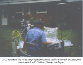
Sample collection and analysis
All samples were collected using the clean sampling procedures specified by
the USGS National Water-Quality Assessment (NAWQA) program (Shelton, 1994).
Unsoftened water samples were collected from domestic wells by connecting to
external, garden hose taps. All tubing used in sample collection was Teflon-lined,
with high-density polyethylene (HDPE) or Teflon fittings and connectors. Physical
characteristics (temperature, specific conductance, dissolved oxygen, pH, eH)
were measured at the well-site with a Hydrolab H20 connected in-line through
a flow-through cell. Before a ground-water sample was collected for laboratory
analysis, wells were purged for a period of at least 20 minutes until the above
field characteristics had stabilized. Stability was determined on the basis
of the following criteria; specific conductance variation less than 2 µS/cm,
pH variation less than 0.05 pH units, dissolved oxygen variation less than 0.05
mg/L, and a temperature variation of less than 1oC. Alkalinity titrations were
performed on filtered samples in the field.
All wells were sampled for analysis of major cations, major anions, nutrients, and arsenic. A complete list of laboratory analyses is included in table 2. The USGS National Water Quality Laboratory (NWQL) in Arvada, Colorado performed all analyses listed in table 2.
At 26 sites, replicate samples were collected for analysis by the MDEQ. These samples were collected to examine the comparability of MDEQ analytical results for arsenic, nitrate, and chloride to results from the USGS NWQL. The MDEQ laboratory uses an inductively coupled plasma mass spectrometry (ICPMS) method for arsenic analyses (MRL = 0.0001 mg/L), and colorimetric methods for nitrate (MRL = 0.4 mg/L) and chloride (MRL = 4 mg/L) analyses.
Five wells were selected to provide information on long-term seasonal variations in ground-water quality. These wells were sampled using methods identical to those described previously for the collection of ground-water-quality samples.
Five wells were sampled to evaluate short-term (0 - 25 minutes) variations in chemical composition of drinking water. Operationally, drinking water is distinguished from ground water by the fact that the well and plumbing system are not purged before sample collection. The sample is thus reflective of what a resident might consume if simply getting a glass of water. Sampling procedures were designed to evaluate potential changes in concentrations of arsenic, manganese, and iron within a domestic plumbing system. Four wells were selected on the basis of detection of arsenic, manganese, and iron in samples analyzed at the NWQL. One well, OAK 41, was added to this sample group because of extensive prior data on record at MDEQ. At wells selected for the short-interval, time-series sample collection, unfiltered samples were collected at intervals ranging from 30 seconds to 2 minutes for the first 20 to 25 minutes of well pumping. Wells were not purged prior to collecting the first sample. These samples were analyzed for total arsenic using a flame atomic absorption method (Brown, 1998). Manganese and iron were analyzed using an ICPMS method (Garbarino and Struzeski, 1998).
Field-Measured Characteristics
Temperature, specific conductance, oxidation-reduction potential (eH), dissolved
oxygen (DO), pH, and alkalinity were measured in the field. Results of these
analyses are shown in appendix table 1B. No health standards exist for any of
these constituents, but the USEPA has issued a Secondary Maximum Contaminant
Level for pH based on aesthetic considerations.
Table 2: Water quality characteristics
analyzed by the USGS National Water Quality Laboratory
[µS/cm, microsiemens
per centimeter at 25 degrees Celsius; °C, degrees Celsius; mg/L, milligrams
per liter]
| Parameter Name | Units | MRL | Parameter Code | Method | Reference |
|---|---|---|---|---|---|
| Specific Conductance | µs/cm | 1 | 90095 | I278185 | Fishman and Friedman, 1989 |
| pH, Laboratory | Standard Units | 0.1 | 403 | I258785 | Fishman and Friedman, 1989 |
| Total Residue @ 180 oC | mg/L | 1 | 530 | I376585 | Fishman and Friedman, 1989 |
| Calcium, dissolved | mg/L as Ca | 0.02 | 915 | I147287 | Fishman and Friedman, 1989 |
| Magnesium, dissolved | mg/L as Mg | 0.004 | 925 | I147287 | Fishman, 1993 |
| Sodium, dissolved | mg/L as Na | 0.06 | 930 | I147287 | Fishman, 1993 |
| Potassium, dissolved | mg/L as K | 0.1 | 935 | I163085 | Fishman and Friedman, 1989 |
| Acid Neutralizing Capacity | mg/L as CaCO3 | 1 | 90410 | I203085 | Fishman and Friedman, 1989 |
| Sulfate, dissolved | mg/L as SO4 | 0.1 | 945 | I205785 | Fishman and Friedman, 1989 |
| Chloride, dissolved | mg/L as Cl | 0.1 | 940 | I205785 | Fishman and Friedman, 1989 |
| Flouride , dissolved | mg/L as F | 0.1 | 950 | I232785 | Fishman and Friedman, 1989 |
| Bromide, dissolved | mg/L as Br | 0.01 | 71870 | I212985 | Fishman and Friedman, 1989 |
| Silica , dissolved | mg/L as SiO2 | 0.1 | 955 | I270085 | Fishman and Friedman, 1989 |
| Residue, dissolved 180oC | mg/L | 10 | 70300 | I175085 | Fishman and Friedman, 1989 |
| Nitrogen, Ammonia, dissolved | mg/L as N | 0.02 | 608 | I252290 | Fishman, 1993 |
| Nitrogen, Nitrite, dissolved | mg/L as N | 0.01 | 613 | I254090 | Fishman, 1993 |
| Nitrogen, Ammonia + Organic | mg/L as N | 0.1 | 623 | I261091 | Patton and Truitt, 1992 |
| Nitrogen, Nitrite + Nitrate, dissolved | mg/L as N | 0.05 | 631 | I254590 | Fishman, 1993 |
| Phosphorus, total | mg/L as P | 0.05 | 665 | I461091 | Patton and Truitt, 1992 |
| Phosphorus, dissolved | mg/L as P | 0.004 | 666 | EPA 365.1 | U.S.EPA, 1993 |
| Phosphorus, Orthophosphate | mg/L as P | 0.01 | 671 | I260190 | Fishman, 1993 |
| Arsenic, total* | mg/L as As | 0.001 | 1002 | I406398 | Brown, 1998 |
| Arsenic, total, EPA | mg/L as As | 0.001 | 1002D | EPA 200.9 | U.S.EPA, 1993 |
| Iron, total* | mg/L as Fe | 0.014 | 1045 | I447197 | Garberino and Struzeski, 1998 |
| Iron, dissolved | mg/L as Fe | 0.01 | 1046 | I147287 | Fishman, 1993 |
| Manganese, total* | mg/L as Mn | 0.003 | 1055 | I447197 | Garberino and Struzeski, 1998 |
| Manganese, dissolved | mg/L as Mn | 0.003 | 1056 | I147287 | Fishman, 1993 |
| * denotes method used for short-interval, time-series sample analysis. |
The temperature of water pumped from wells during sampling ranged from 10.4oC to 15.5oC, with a mean of 12oC (approximately 54oF). The annual average daily air temperature for the Pontiac area is between 9 and 10oC (Soil Conservation Service, 1982). Ground-water temperatures are usually 1 to 2oC higher than the mean annual air temperature (Todd, 1980).
The concentration of dissolved solids in water can be approximated in the field by measuring the specific conductance of a sample (Hem, 1985). Fresh water is usually considered to be water containing less than 1,000 mg/L total dissolved solids (Drever, 1988). The USEPA SMCL for dissolved solids is 500 mg/L. On the basis of data collected in this study, the total dissolved solids concentration in ground water in Oakland County [in milligrams per liter (mg/L)] is typically about 58 percent of the specific conductance [measured in microsiemens/centimeter (µS/cm)]. Thus, the threshold between fresh and brackish water in Oakland County would be represented by a specific conductance of approximately 1,800 µS/cm, and the USEPA's SMCL would be represented by a specific conductance of approximately 900 µS/cm. The specific conductance of ground water used for drinking in Oakland County ranged from 395 to 2,950 µS/cm, with a mean value of 925 µS/cm.
Dissolved oxygen concentrations ranged between <0.1 and 7.8 mg/L, with a mean of 0.8 mg/L. In Michigan, the presence of DO in concentrations higher than 1.0 mg/L is typically associated with recently recharged, and usually shallow, ground water. The concentration of dissolved oxygen in the water, along with the oxidation-reduction potential (redox), controls the chemical and microbial reactions that can occur in ground water.
The pH of ground water in Oakland County varies between 6.5 and 7.6, with a mean of 7.1. Most ground water in the United States falls in the range of 6.0 to 8.5 (Hem, 1985). The USEPA SMCL for pH specifies pH should fall between 6.5 and 8.0.
The redox potential of Oakland County ground water ranged from -25mV to 876mV. The redox potential is not directly related to any health effects; rather, it is monitored as an indication of whether the subsurface environment is conducive to removing electrons from materials (high eH) or adding electrons to material (low eH). Higher eH values are often found in recently recharged waters, while lower eH values are found in older waters that have been exposed to more organic matter, carbonates, or bacteria (Drever, 1988). The redox potential of water is an important control on geochemical processes, and the determination of eH can indicate which ions are likely to be mobile in the system. The measurements included in appendix table 1B and elsewhere are approximate, based on results from an electrode measurement, rather than direct measurement of different species of the same ion.
The alkalinity of ground water in Oakland County ranged from 214 to 462 mg/L as CaCO3-. Alkalinity is a measure of the acid neutralizing ability of a sample, which can be the result of several ions in solution. In the pH ranges described above, the principal ion responsible for alkalinity is bicarbonate, HCO3- (Hem, 1985). Like the redox potential, alkalinity is an indicator of the state of the geochemical system, and aids in the interpretation of other chemical constituents.
Inorganic Chemical Constituents
The USEPA has set drinking-water MCLs and SMCLs for several inorganic constituents
analyzed in this study. These constituents, the USEPA threshold, and the type
of threshold are shown in table 3 (U.S. Environmental Protection Agency, 1996).
A complete list of inorganic chemistry analyses can be found in appendix table
1C. A summary of results for each inorganic constituent are shown in table 4.
Table 3. Inorganic constituents analyzed
in this study with USEPA Drinking Water Standards
[mg/L, milligrams per liter; MCL, Maximum Contaminant Level; SMCL, Secondary
Maximum Contaminant Level]
| CONSTITUENT | LIMIT | UNITS | STANDARD TYPE |
|---|---|---|---|
| Nitrite | 1 | mg/L as N | MCL |
| Nitrate | 10 | mg/L as N | MCL |
| Chloride | 250 | mg/L as Cl | SMCL |
| Sulfate | 250 | mg/L as SO4- | SMCL |
| Flouride | 4 | mg/L as F | SMCL |
| Arsenic | 0.05 | mg/L as As | MCL |
| Iron | 0.3 | mg/L as Fe | SMCL |
| Manganese | 0.05 | mg/L as Mn | SMCL |
| Total Dissolved Solids | 500 | mg/L | SMCL |
Table 4. Summary statistics for selected
inorganic constituents detected in water samples from selected wells in Oakland
County, Michigan
[mg/L, milligrams per liter; µg/L, micrograms per liter; µS/cm, microsiemens
per centimeter at 25oC]
| Maximum | Minimum | Mean | Median | |
|---|---|---|---|---|
| Laboratory pH (Standard Units) | 7.9 | 7.1 | 7.42 | 7.43 |
| Nitrogen, Ammonia (mg/L as N) | 1.4 | <.02 | 0.19 | 0.14 |
| Nitrogen, Nitrite (mg/L as N) | 0.1 | <.01 | 0.01 | <.01 |
| Nitrogen, Ammonia + Organic (mg/L as N) | 1.52 | <.01 | 0.22 | 0.15 |
| Nitrogen, Nitrate + Nitrite, dissolved (mg/L as N) | 23.9 | <.05 | 0.9 | <.05 |
| Phosphorus, dissolved (mg/L as P) | 0.5 | <.004 | 0.02 | <.004 |
| Phosphorus, ortho (mg/L as P) | 0.5 | <.01 | 0.02 | <.01 |
| Calcium, dissolved (mg/L as Ca) | 175 | 0.15 | 79.3 | 76.2 |
| Magnesium, dissolved (mg/L as Mg) | 57.7 | 0.02 | 29 | 27.5 |
| Sodium, dissolved (mg/L as Na) | 431 | 3.73 | 66 | 22.8 |
| Potassium, dissolved (mg/L as K) | 13 | 0.1 | 2.1 | 1.7 |
| Chloride, dissolved (mg/L as Cl) | 661 | 0.48 | 103 | 23.3 |
| Sulfate, dissolved (mg/L as SO4-) | 80.7 | 1.26 | 29.8 | 18.5 |
| Flouride, dissolved (mg/L as F) | 1.1 | <.1 | 0.4 | 0.2 |
| Silica, dissolved (mg/L as SiO2) | 23 | 9.25 | 14.7 | 14.3 |
| Arsenic, total (mg/L as As) | 0.176 | <.001 | 0.021 | 0.003 |
| Iron, dissolved (mg/L as Fe) | 3.58 | <.014 | 1.09 | 0.927 |
| Manganese, dissolved (mg/L as Mn) | 0.33 | <.003 | 0.055 | 0.032 |
| Dissolved Residue of Evaporation, 180oC (mg/L) | 1620 | 228 | 529 | 387 |
| Bromide, dissolved (mg/L as Br) | 5.5 | 0.01 | 0.24 | 0.06 |
| Specific Conductance, (µs/cm) | 2950 | 408 | 913 | 640 |
None of the samples contained concentrations of sulfate or fluoride in excess of the SMCL. Samples from two wells exceeded the MCL for nitrate. Samples from more than half of the wells contained concentrations of iron in excess of the SMCL, and samples from nearly half of the wells contained concentrations of manganese in excess of the SMCL. Concentrations of arsenic in samples from five wells exceeded the MCL; although all of those wells were previously identified by MDEQ as having concentrations above the MCL. Samples from seven wells exceeded the SMCL for chloride. Samples from twelve wells exceeded the SMCL for total dissolved solids.
Elevated concentrations of iron, manganese, and arsenic are associated with ground water with lower redox potential at near-neutral pH (Hem, 1985; Kim, 1999; Korte and Fernando, 1991). This association can be observed in wells in Oakland County. However, nitrate and nitrite are readily reduced to nitrogen in low-redox environments. Appropriately, nitrate and nitrite were not present in any well with a concentration of arsenic, manganese, or iron in excess of the USEPA standard. Consumption of water with iron or manganese concentrations above the SMCL is not considered dangerous from a health perspective; however, both materials leave deposits in pipes and on fixtures, impart taste to beverages, and can discolor laundry (Shelton, 1997).
Sulfur is a common element in the Earth's crust, and occurs as sulfate (SO42-) in waters with near-neutral pH and redox potential above -100 mV (Hem, 1985). Sulfate can be reduced under certain conditions to hydrogen sulfide, a compound with the smell of rotten eggs. In addition to leaving greenish deposits on plumbing fixtures, sulfate in concentrations above the SMCL can result in diarrhea (Shelton, 1997).
Fluoride is present in many natural waters in concentrations less than 1.0 mg/L. The MCL of 4.0 mg/L has been set to protect public health. Fluoride in excess of 4.0 mg/L can cause skeletal fluorosis, a serious bone disorder (Shelton, 1997). Concentrations in excess of 2.0 mg/L can cause dental fluorosis, a staining and pitting of the teeth (Shelton, 1997).
The SMCL for dissolved solids is based on aesthetic concerns, and is primarily related to the life expectancy of domestic plumbing and appliances. The service life for a hot water heater is reduced by one year for every 200 mg/L of dissolved solids in water above the average 220 mg/L (Shelton, 1997).
Nutrients
Species of nitrogen and phosphorus are frequently referred to as nutrients,
because they are essential to plant life and are common in fertilizers, including
manure, and in human waste. There are no health restrictions on consumption
of phosphorus in drinking water, but the USEPA has set restrictions on nitrate
(NO3-) and nitrite (NO2-).
Sources
Nitrogen and phosphorus are essential to all known forms of life. Consequently,
they can be found throughout the environment in varying concentrations, even
in rainwater. Typical nitrate concentrations in the precipitation of southwestern
Michigan are approximately 0.6 mg/L as N, and typical phosphorus concentrations
are 0.05 mg/L (Cummings, 1978).
Human activities have done much to alter the distribution of nutrients in the environment. Application of manure and chemical fertilizers to crops and lawns results in local abundance of nutrients, which is the desired outcome. But over-application can result in local excesses of nutrients, which can reach ground water. Septic tanks are designed to provide a means of containing and treating sewage, which typically contains elevated concentrations of nitrogen and phosphorus. But when environmental conditions, such as a high water table, alter the operation of a septic tank, nitrogen and phosphorus can be released into the ground water. The USEPA considers nitrate concentrations of 3 mg/L as N or higher to be the result of anthropogenic contamination (U.S. Environmental Protection Agency, 1996b).
Occurrence
Concentrations of nitrate and nitrite in Oakland County drinking water ranged
from below the reporting limit (0.1 mg/L) to 23.9 mg/L as N, more than twice
the MCL. Samples collected from two wells exceeded the MCL, although samples
from three more wells contained concentrations greater than 2 mg/L as N. While
not above the USEPA threshold for anthropogenic contamination, these concentrations
are more than twice the median, and more than three times the atmospheric loading.
Nitrite concentrations were consistently less than the MCL of 1.0 mg/L as N,
ranging from 0.08 to less than the reporting limit of 0.01 mg/L as N.
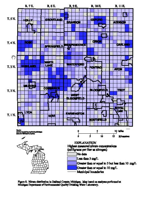
The CAER used 6,198 of the 12,942 nitrate analyses performed by MDEQ to generate the map of nitrate occurrence in Oakland County (fig. 8). The majority of the discarded records were removed because of obvious errors in recording the address in the database. In the case of duplicate entries for a well, the highest concentration was retained. Each of the 900 survey sections in Oakland County was then assigned to one of four groups; nitrate present above the MCL, nitrate present below the MCL, nitrate present below 3 mg/L-N, or no observations. Approximately one percent (96) of the 7,814 unique wells identified by the CAER contained concentrations of nitrate greater than the MCL. A more detailed discussion of the mapping methods employed and the comparison between USGS analytical results and MDEQ analytical results is included in Appendix 2.
The map provides a summary of the nitrate data in the MDEQ database. Nitrate concentrations above 3 mg/L-N generally occur along a northeast-southwest axis, coincident with the region previously identified as both the interlobate outwash plains and the region of with the most permeable soils (see figure 5). This pattern of nitrate contamination of ground water through high permeability surface sediments has been widely documented in Michigan (Kittleson, 1987) and elsewhere (Madison and Brunett, 1985).
Nitrate concentrations in ground water change at spatial scales smaller than the square-mile mapping unit used in these maps. The classification applied to any square-mile mapping unit does not necessarily reflect the current status of all wells in that mapping unit. The data archived in the MDEQ database reflect analyses of samples collected between 1983 and 1997, with varying sample collection, handling, and analysis techniques. For example, replicate samples collected in this study, and some samples collected by state and county personnel, employed clean sampling techniques to minimize contamination. Samples in this study (excluding the short-interval samples, discussed later), as well as samples collected by state and county workers, were collected only after the well and plumbing system had been purged. Samples were returned to the state laboratory the same day for analysis within the next two days. The majority of the samples in the MDEQ database, however, were collected by homeowners and shipped by mail to the State laboratory for analysis. Thus there is no standard control on sampling procedures, handling techniques, or the time elapsed between sample collection and analysis.
Potential Health Effects
Nitrate has long been linked to methemoglobinemia in infants (Comly, 1945),
commonly known as "blue baby syndrome." Methemoglobinemia occurs when
nitrite (NO2-), a reduced form of nitrate, interacts with red blood cells and
impairs their ability to carry oxygen (Mirvish, 1991). This impairment results
in anoxia (deficiency of oxygen in the blood) and cyanosis (blue blood). In
severe cases, blue-baby syndrome can be fatal (U.S. Environmental Protection
Agency, 1996b). Susceptibility varies depending on age, body mass, and diet,
but fetuses and infants under 6 months are most at risk. This is because 1)
infantile hemoglobin is more susceptible to oxidation by nitrite than adult
hemoglobin, 2) infants consume more water per unit body weight than do adults,
and 3) the activity of the enzyme system that removes methemoglobin in infants
is lower in infants than in adults (Keeney and Follett, 1991). For this reason,
the USEPA has set restrictions on nitrate (NO3-) and nitrite
(NO2-) concentrations
of 10.0 and 1.0 mg/L as nitrogen, respectively (U.S. Environmental Protection
Agency, 1996a). Most laboratories report nitrate and nitrite concentrations
in terms of the weight of nitrogen (as above). In terms of the mass of the whole
molecule, the MCLs are approximately 45 mg/L as NO3- and 3.3 mg/L as NO2-.
Several authors (Keeney, 1986; Keeney and Follett, 1991; Moller and Forman, 1991; Crespi and Ramazotti, 1991) have accepted the correlation between nitrate consumption and various forms of cancer. Nitrosamines, formed from ingested nitrite and amines, which occur naturally in the digestive tract, also have been identified as carcinogens in laboratory experiments (Crespi and Ramazotti, 1991). Because nitrate and nitrite can be ingested from other sources, such as food and wine, no evidence currently exists for evaluating potential carcinogenic effects of nitrate on human populations (Crespi and Ramazotti, 1991).
Major Ions and Trace Metals
In addition to nutrients, water samples from the wells in Oakland County were
analyzed for more than a dozen other characteristics. Summary statistics are
provided in table 4. The complete listing of these results is included in appendix
tables 1A to 1G. A more detailed description of the sources, occurrence, and
health effects of chloride and arsenic has been developed to assist county employees
and citizens in making decisions about drinking-water resources.
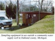
Image of: Collection of water samples for analysis, Oakland county, Michigan. (122 KB)
Chloride
Chloride is found in virtually all ground water. Chloride can occur in ground
water naturally, but is also found throughout southeastern Michigan as the result
of human activities (Thomas, in press). The principal natural source of chloride
in ground water is seawater trapped within the rock matrix (Long and others,
1986). Several anthropogenic sources exist as well, including the salts used
on roads for deicing and dust control, and water softeners. Chloride is a conservative
ion in solution, and seldom interacts in organic or inorganic reactions in the
subsurface (Hem, 1985). As a result, the evidence of anthropogenic additions
of chloride may be present for many years.
Occurrence
Samples collected from 7 of the 37 wells exceeded the SMCL for chloride. Samples
from every well contained a detectable concentration of chloride, ranging from
0.48 mg/L to 661 mg/L. The mean concentration was 104 mg/L and the median concentration
was 23 mg/L.
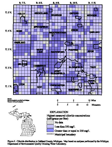
The CAER used 6,228 of the 12,960 chloride analyses performed by MDEQ to generate the map of chloride occurrence in Oakland County (fig. 9). The majority of the discarded records were removed because of obvious errors in the database. In the case of duplicate entries for a well, the highest concentration was retained. Each of the 900 survey sections in Oakland County was then assigned to one of four groups; chloride present above the SMCL, chloride present below the SMCL, chloride present below the MRL, or no observations. Approximately 5 percent (383) of the 7,809 unique wells identified by the CAER contained chloride in concentrations greater than the SMCL of 250 mg/L. Of the unique wells identified from the database, 1,581 did not have sufficient address location data to place them accurately on the map. A more detailed discussion of the mapping methods employed and the comparison between USGS analytical results and MDEQ analytical results is included in Appendix 2.
This map provides a summary of the chloride data in the MDEQ database. Because elevated chloride concentrations in ground water can come from both anthropogenic and natural sources, elevated chloride concentrations can be found throughout the county. Chloride concentrations in ground water can change at spatial scales smaller than the square-mile mapping unit used in these maps. The classification applied to any square-mile mapping unit does not necessarily reflect the current status of all wells in that mapping unit.
The data archived in the MDEQ database reflect analyses on samples collected between 1983 and 1997, with varying sample collection, handling, and analysis techniques. For example, replicate samples collected in this study, and some samples collected by state and county personnel, employed clean sampling techniques to minimize contamination. Samples in this study (excluding the short-interval samples, discussed later), as well as samples collected by state and county workers, were collected only after the well and plumbing system had been purged. The majority of the samples in the MDEQ database, however, were collected by homeowners and shipped by mail to the State laboratory for analysis. Thus there is no standard control on sampling procedures, handling techniques, or the time elapsed between sample collection and analysis.
Potential Health Effects
Hutchinson (1970) suggested that elevated chloride concentrations could have
an effect on persons with pre-existing cardiac (heart) or renal (kidney) problems.
The chloride SMCL of 250 mg/L is based on the aesthetic consideration of taste;
water with higher concentrations of chloride tastes 'salty' to most people.
A greater concern might be the presence of cations with chloride, such as sodium
and potassium. Sodium in drinking water can be a concern for those on low sodium
diets because of cardiac, circulatory, renal or other problems (Shelton, 1997).
Arsenic
Arsenic is a common element in the Earth's crust, and occurs naturally throughout
southeastern Michigan in several forms. In ground water, arsenic has been observed
to occur in two forms; the oxidized form, arsenate (As5+), or the reduced form,
arsenite (As3+). Kim (1999), working with the USGS Drinking Water Initiative
(DWI) project, has shown that most (65-94 percent) of the arsenic in ground
water in Oakland County is arsenite. Kim (1999) has also observed that the presence
of the bicarbonate ion (HCO3-) in solution can enhance the rate of arsenic dissolution
into ground water, although the species of arsenic released by this process
is arsenate. Arsenate is readily sorbed to metal oxides, such as iron oxide,
and rendered immobile (Korte and Fernando, 1996). For arsenic to be released
into solution from the mineral form, arsenian pyrite (Kolker and others, 1998),
aquifer sediments must first be oxidized, then reduced. The hydrologic mechanism
facilitating this process has not yet been determined.
Occurrence
Low concentrations of arsenic are found throughout southeastern Michigan. The
largest concentration detected in Oakland County by this study was 0.175
mg/L. Samples from five of the 38 wells exceeded the MCL, 0.05 mg/L, although
all had previously been noted to exceed the MCL based on results from the MDEQ
laboratory and were sampled to obtain additional supporting chemistry. Of the
other wells sampled, 9 contained arsenic in concentrations below the minimum
reporting level of 0.001 mg/L. The remaining 24 wells all contained some detectable
concentration between 0.001 and 0.050 mg/L.
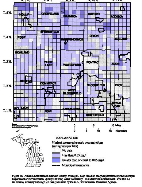
The CAER used 1,988 of the 3,509 arsenic analyses performed by MDEQ to generate the map of arsenic occurrence (fig. 10) using procedures similar to those described for nitrate and chloride. These maps are similar to those released previously in USGS Fact Sheet 135-98 (Aichele and others, 1998). Approximately one percent (24) of the 2,373 unique wells identified by the CAER contained arsenic at concentrations greater than the MCL of 0.05 mg/L. Of the unique wells identified from the database, 385 did not have sufficient address location data to place them accurately on the map. A more detailed discussion of the mapping methods employed and the comparison between USGS analytical results and MDEQ analytical results is included in Appendix 2.
The map provides a summary of the arsenic data in the MDEQ database. Arsenic concentrations in ground water can change at spatial scales smaller than the square-mile mapping unit used in these maps. The classification applied to any square-mile mapping unit does not necessarily reflect the current status of all wells in that mapping unit.
The data archived in the MDEQ database reflect analyses on samples collected between 1983 and 1997, with varying sample collection, handling, and analysis techniques. For example, replicate samples collected in this study, and some samples collected by state and county personnel, employed clean sampling techniques to minimize contamination. Samples in this study (excluding the short-interval samples, discussed later), as well as samples collected by state and county workers, were collected only after the well and plumbing system had been purged. The majority of the samples in the MDEQ database, however, were collected by homeowners and shipped by mail to the State laboratory for analysis. Thus there is no standard control on sampling procedures, handling techniques, or the time elapsed between sample collection and analysis.
Potential health effects
The USEPA has set an MCL of 0.05 mg/L for arsenic in drinking water, although
no distinction is made between the two arsenic species. In May, 2000 the USEPA
proposed revising the MCL to 0.005 mg/L, and is accepting public comment on
MCLs of 0.003 mg/L, 0.005 mg/L, 0.010 mg/L, and 0.020 mg/L. A final decision
is expected early in 2001.
Several authors have suggested that arsenite may be a more serious health concern than arsenate (Pontius and others,1994; Kosnett, 1997). The effects of chronic arsenic ingestion are based on the total daily dose and length of exposure, not the concentration specifically. The daily dosage from drinking water can be estimated based on the concentration in the water and the quantity of water consumed. For example:
[As concentration] * Quantity of = Dose of water
0.050 mg/L * 2 L = 0.100 mg
0.025 mg/L * 2 L = 0.050 mg
This calculation is only an estimate of total daily arsenic ingestion, because there are other environmental sources of arsenic. Some of these sources include shellfish, meats, dust, soil, and some pigments. The U.S. Food and Drug Administration has estimated that US adults ingest about 0.053 mg As/day from the diet, not including drinking water (Guo and others, 1998). Nearly half of this amount comes from fish and shellfish. Marine shellfish and cod typically contain arsenic concentrations between 10 and 40 mg/kg based on fresh weight (National Academy of Science, 1977). Freshwater fish, other marine fish, pork and beef typically contain less than 1 mg As/kg (National Academy of Science, 1977).
Kosnett (1997) defines three classes of arsenic exposure, and outlines the symptoms and risks associated with each class. For an average adult, low exposure includes inorganic arsenic doses up to 0.5 mg/day. Moderate exposure includes dose of 0.5 to 1.5 mg/day, and high exposures are doses in excess of 1.5 mg/day. These exposure classes are based on the total mass of arsenic ingested from water (described above) and from food. Low doses seldom result in any noticeable symptoms of illness. Moderate exposures for prolonged periods (5 to 15 years) may result in skin discoloration and lesions, anemia, peripheral neuropathy and peripheral vascular disease. In addition to the symptoms of moderate exposure, high doses may result in edema, more pronounced peripheral neuropathy including motor weakness, diminished reflexes, and muscle atrophy. High doses also may result in gastrointestinal disturbances such as nausea and diarrhea, as well as general fatigue and weight loss.
Arsenic has been listed as a Group A human carcinogen by the USEPA on the basis of inhalation and ingestion exposure. The carcinogenic effects of low-level arsenic ingestion in drinking water are widely disputed in the medical literature and are currently under review by the USEPA. Several case studies of groups exposed to arsenic occupationally or medicinally, such as Moselle wine growers (Luchtrath, 1983) and users of the Victorian health tonic 'Fowler's solution,' an alkaline solution of potassium arsenate marketed in the US until 1980, have indicated increased risks of bladder cancers (Cuzick and others, 1992). Several studies in Taiwan (Tsuda and others, 1995; Pontius and others, 1994) have observed increased risk of urinary tract cancers as a result of consuming water containing arsenic. No statistically significant relation was observed between arsenic concentration in drinking water and the occurrence of liver, kidney, bladder, or urinary tract cancer for persons consuming water containing less than 0.33 mg/L in Taiwan (Guo and others, 1998).
Different populations may also have different processes to remove arsenic from the body. Most mammals remove arsenic from their bodies by incorporating the arsenic into organic compounds, a process known as methylation. These organic compounds are easier for the body to remove. Dr. Vasken Aposhian of the University of Arizona has determined that several South American mammals have developed a means of removing arsenic from the body other than methylation (Kaiser, 1998). Several native human populations in the Andes Mountains exhibit a similar trait (Kaiser, 1998). Despite drinking water with levels of arsenic more than twice the USEPA MCL, these populations do not exhibit any increased occurrence of cancer (Kaiser, 1998).
At this point, no comprehensive epidemiological study has been performed on a US population consuming arsenic in drinking water over an extended period of time. The best information available comes from studies in Taiwan and Bangladesh, whose populations differ sharply from United States populations in lifestyle, diet, and genetic inheritance.
Results of Time-Series Analyses
Analyses of well water samples collected by the Oakland County Health Division
and homeowners as part of routine sampling have indicated changes in arsenic
concentration of as much as 0.05 mg/L or more over periods of time ranging from
days to years. This variation has raised concerns that 1) concentrations of
arsenic and other dissolved constituents may be changing in the aquifer, or
that 2) some samples may have been collected without an adequate well purge.
An inadequate well purge would mean that drinking water (water drawn from a
tap immediately) was being compared to ground water (water drawn after the plumbing
system and well bore have been purged). As part of this study, ground-water
samples were collected from selected wells to attempt to observe long-term variability
in the aquifer, while drinking-water samples were collected to evaluate the
potential to obtain varying results based on an inadequate purging of the well.
Very little change was observed in any characteristic between ground-water samples collected in June/July 1998 and those collected in December 1998.
All sites exhibited some chemical changes in the short-term drinking-water sampling (Appendix table 1E-1G). Total iron concentrations fluctuated with time in all wells, although the magnitude of the fluctuation was usually less than 10 percent of the concentration. OAK 35 exhibited a marked increase in iron and arsenic concentration over time. Iron concentrations increased from 216 to 1500 µg/L over a span of 10 minutes. Arsenic concentrations increased from 0.001 mg/L to 0.01 mg/L over a time span of four minutes. This sample was collected from a tap at an outbuilding that had not been used for more than two days. This point was sampled because, based on the chemistry data collected earlier, this well was expected to exhibit a short-term change. Improper purging of a well prior to sampling may result in lower concentrations of both arsenic and iron, particularly when the water has been standing in the pipes for a prolonged period.
Results of Replicate Sample Analysis
The analytical results from the USGS NWQL and the MDEQ Drinking Water Laboratory
for nitrate, chloride, and arsenic agree closely. Mean differences in concentration
measurements for nitrate, chloride, and arsenic were 0.1, 6.8, and 0.0008 mg/L,
respectively. The standard deviation of the differences was 0.3, 9.6, and 0.003
mg/L for nitrate, chloride, and arsenic, respectively. Graphs showing the comparative
analytical results over a range of concentrations are provided in
Appendix 2.
SUMMARY
The quality of ground water in Oakland County is the result of a combination
of natural and anthropogenic processes. Many wells produce highly reduced water
with high concentrations of iron and manganese. All of the wells sampled during
1998 contained chloride, although most contained concentrations below the U.S.
Environmental Protection Agency (USEPA) Secondary Maximum Contaminant Level
(SMCL). Twenty-nine of thirty-eight wells contained detectable concentrations
of arsenic, although only five contained arsenic concentrations above the USEPA
Maximum Contaminant Level (MCL). These five wells are best considered separately,
because they were known from previous samplings to contain arsenic, and were
sampled to provide additional chemical information. Only two wells contained
nitrate in concentrations above the MCL, although three additional wells contained
concentrations several times higher than would be expected to be found in precipitation.
Seasonal variations in water-quality were not observed in any of the five wells resampled in December 1998. Some short-term variations during the purging of the wells were observed in all wells. All wells exhibited variation in iron concentration; three of five exhibited fluctuations of approximately 10 percent, while 2 of the five exhibited increasing trends. One well exhibited an increasing trend in arsenic concentration, coincident with an increasing trend in iron concentration. Thus, while in many cases analytical results may not be affected by the length of time a well is purged, in at least one of the five subject wells purge time would have influenced the resulting arsenic concentration.
REFERENCES CITED
Aichele, Steve, Hill-Rowley, Richard, and Malone, Matt, 1998, Arsenic, Nitrate,
and Chloride in Groundwater, Oakland County, Michigan: U.S. Geological Survey
Fact Sheet 135-98, 6 p.
Blumer, S.P., Behrendt, T.E., Ellis, J.M., Minnerick, R.J., LeuVoy, R.L., and
Whited, C.R., 1998, Water Resources Data for Michigan, Water Year 1998: U.S.
Geological Survey Water-Data Report MI-98-1, 477 p.
Britton, L.J., and Greeson, P.E., 1988, Methods for collection and Analysis
of Aquatic Biological and Microbiological Samples: U.S. Geological Survey Techniques
of Water Resources Investigations, Book 5, Chapter A4, 363 p.
Brown, G.E., 1998, Graphite Furnace Atomic Adsorption Spectrophotometry (GFAAS)
to replace Hydride Generation Atomic Adsorption Spectrophotometry (HGAAS) for
the determination of Arsenic and Selenium in Filtered and Whole Water Recoverable
Water, and Recoverable Bottom Material Sediment: U.S. Geological Survey Technical
Memorandum 98.11, 2 p.
Comly, H.H., 1945, Cyanosis in infants caused by nitrates in well-water: Journal
of the American Medical Association, vol. 129, p.112-116.
Crespi, M. and Ramazotti, V., 1991, Evidence that N-nitroso compounds contribute
to the causation of certain human cancers, in Bogardi, I. and Kuzelka, R. (eds.)
Nitrate Contamination: Exposure, Consequence and Control: Springer-Verlag, New
York, p. 233-253.
Cummings, T.R., 1978, Agricultural Land Use and Water Quality in the Upper St.
Joseph River Basin, Michigan: U.S. Geological Survey Open-File Report 78-950,
106 p.
Cuzick, J., Saaieni, P., and Evans, S., 1992: Ingested Arsenic, Keratosis, and
Bladder Cancer: American Journal of Epidemiology, vol. 136, p. 417-412.
Drever, J.I., 1988. The Geochemistry of Natural Waters, 2nd Edition: Prentice
Hall, Inc., Englewood Cliffs, New Jersey, 402 p.
Environmental Systems Research Institute, 1998, Introduction to ArcView GIS:
Environmental Systems Research Institute, Inc., Redlands, California.
Eschman, D.F., and Karrow, P.F., 1985, Huron Basin Glacial Lakes: A Review,
in Karrow, P.F., and Calkin, P.E., Quaternary Evolution of the Great Lakes:
Geological Association of Canada, Special Paper 30, p. 79-94.
Ferrand, W.R., and Bell, D.L., 1982, Quaternary Geology of Southern Michigan:
Michigan Geological Survey, 1:500,000 scale, 2 sheets.
Fetter, C.W., 1994, Applied Hydrogeology, 3rd ed.: Macmillan College Publishing,
Inc., New York, 616 p.
Fishman, M.J., and Friedman, L.C., 1989, Methods for determination of inorganic
substances in water and fluvial sediments: U.S. Geological Survey Techniques
of Water Resources Investigations, Book 5, Chapter A1, 454 p.
Fishman, M.J., 1993, Methods of Analysis of the U.S. Geological Survey National
Water Quality Laboratory - Determination of inorganic and organic constituents
in water and fluvial sediments: U.S. Geological Survey Open-File Report 93-125,
273 p.
Garbarino, J.R., and Struzeski, T.M., 1998, Methods of analysis by the U.S.
Geological Survey National Water Quality Laboratory -- Determination of elements
in whole-water digests using inductively coupled plasma-optical emission spectrometry
and inductively coupled plasma-mass spectrometry: U.S. Geological Survey Open-File
Report 98-165, 101 p.
Guo, H.R., Chiang, H.S., Hu, H., Lipsitz, S.R., and Monson, R.R., 1998, Arsenic
in Drinking Water and incidence of Urinary Tract Cancers: Epidemiology, vol.
8, no. 5, p. 545-550.
Hem, J.D., 1985, Study and Interpretation of the Chemical Characteristics of
Natural Water, 3rd Edition: U.S. Geological Survey Water-Supply Paper 2254,
249 p.
Holtschlag, D.J., and Nicholas, J.R., 1998, Indirect Ground-water discharge
to the Great Lakes: U.S. Geological Survey Open-File Report 98-579, 25 p.
Humphrys, C.R., and Green, R.F., 1962, Michigan Lake Inventory: Michigan State
University Department of Resource Development, Bulletin 63, p. 63A-63H.
Hutchinson, F.E., 1970, Environmental pollution from highway deicing compounds:
Journal of Soil and Water Conservation, vol. 25, p. 144-146.
Kaiser, J., 1998, Toxicologists shed new light on old poisons: Science, vol.
279, p. 1850.
Keeney, D., 1986, Sources of nitrate to ground water: CRC Critical Reviews in
Environmental Control, vol. 16, no. 3, p. 257-304.
Keeney, D. and Follett, R., 1991, Managing nitrogen for ground-water quality
and farm profitability: Soil Science Society of America, Madison, Wisconsin.
357 p.
Kim, M.J., 1999, Arsenic Dissolution and Speciation in Ground water in Southeast
Michigan: Ann Arbor, University of Michigan, Doctoral Dissertaion, 202 p.
Kittleson, K., 1987, The groundwater problem in Michigan: an overview in D'Itri,
F., and Wolfson, L. (eds.), Rural groundwater gontamination: Lewis Publishers,
Chelsea, Michigan, p. 69-84.
Kolker, A., Cannon, W.P., Westjohn, D.B., and Woodruff, L., Arsenic-rich Pyrite
in the Mississippian Marshall Sandstone: Source of Anomalous Arsenic in Southeastern
Michigan Drinking Water [abs.]: Geologic Society of America Abstracts with Programs,
vol. 30, no. 7, p. A-59.
Korte, N.E., and Fernando, Q., 1991, A review of arsenic (III) in ground water:
Critical Reviews in Environmental Control, vol. 21, no. 1, p. 1-39.
Kosnett, M., 1997, Clinical Guidance in the evaluation of patients with potential
exposure to arsenic in drinking water: Michigan Department of Community Health,
Lansing, Michigan, 10 p.
Leverett, F., and others, 1906, Flowing Wells and Municipal Water Supplies in
the Southern Portion of the Southern Peninsula of Michigan: U.S. Geological
Survey Water-Supply Paper 182, 292 p.
Leverett, F., and Taylor, F.B., 1915, The Pleistocene of Indiana and Michigan
and the History of the Great Lakes: U.S. Geological Survey Monograph 53, 529
p.
Long, D.T., Rezabek, T.P., Takacs, M.J., and D.H.,Wilson, 1986, Geochemistry
of ground waters, Bay County, Michigan: Report to Michigan Department of Public
Health and Michigan Department of Natural Resources (MDPH: ORD 385553), 265
p.
Luchtrath, H., 1983, The consequences of chronic arsenic poisoning among Moselle
wine growers: Journal of Cancer Research and Clinical Oncology, vol. 105, p.
173-182.
Madison, R.J., and Brunett, J.O., 1985, Overview of the occurrence of nitrate
in ground water of the United States: U.S.Geological Survey Water-Supply Paper
2275, 105 p.
Mirvish, S.S., 1991, The significance for human health of nitrate, nitrite,
and N-nitroso compounds, in Bogardi, I. and Kuzelka, R. (eds.), Nitrate Contamination:
Exposure, Consequence and Control: Springer-Verlag, New York, p. 253-266.
Moller and Forman, 1991, Epidemiological Studies of the endogenous formation
of N-nitroso compounds, in Bogardi, I. and Kuzelka, R. (eds.), Nitrate Contamination:
Exposure, Consequence and Control: Springer-Verlag, New York, p. 276-280.
Mozola, A.J., 1954, A Survey of the Ground-water Resources in Oakland County,
Michigan: Michigan Department of Conservation, Publication 48, Part II, 348 p.
National Academy of Science, 1977, Drinking Water and Health: National Academy
Press, Washington D.C.
Patton, C.J., and Truitt, E.P., 1992, Methods of Analysis of the U.S. Geological
Survey National Water Quality Laboratory - Determination of total phosphorus
by a Kjeldahl digestion method and an automated colorimetric finish that includes
dialysis: U.S. Geological Survey Open-File Report 92-146, 39 p.
Pontius, F. Brown, K, and Chen, C., 1994, Of arsenic in drinking water: Journal
of the American Water Works Association, vol. 86, no. 10, p. 52-63.
Southeast Michigan Council of Governments, 1995, Land Use/Land Cover, Southeast
Michigan, 1995 - Geographic Information Systems Data Set, Nominal Scale 1:175,000:
Southeast Michigan Council of Governments, Detroit, Michigan.
Southeast Michigan Council of Governments, 1999, 1999 Southeast Michigan Population
and Household Estimates: Southeast Michigan Council of Governments, Detroit,
Michigan, 1 sheet.
Shelton, L.R., 1994, Field guide for collecting and processing stream water
samples for the National Water Quality Assessment Program: U.S. Geological Survey
Open-File Report 94-455, 42 p.
Shelton, T.B., 1997, Interpreting Drinking Water Quality Analysis: What do the
numbers mean? 5th ed.: Rutgers Cooperative Extension Publication E214, New Brunswick,
New Jersey, 67 p.
Soil Conservation Service, 1982, Soil Survey of Oakland County, Michigan: U.S.
Department of Agriculture, Soil Conservation Service, Washington D.C., 162 p.
Thomas, M.A., The Effect of Recent Residential Development on the Quality of
Ground Water near Detroit, Michigan. Accepted for publication in Ground Water
[in press].
Todd, D.K., 1980, Groundwater Hydrology, 2nd ed.: John Wiley and Sons, New York,
516 p.
Tsuda, T., Babazono, A., Yamamoto, E., Kurumatani, N., Mino, Y., Ogawa, T.,
Kishi, Y., Aoyama, H., 1995, Ingested arsenic and internal cancer, a historical
cohort study followed for 33 years: American Journal of Epidemiology, vol. 141,
p. 198-209.
U.S. Environmental Protection Agency, 1994, Methods for the Determination of
Inorganic Substances in Environmental Samples: National Technical Information
Service PB94-120821, 169 p.
_________, 1996a, Drinking Water Regulation and Health Advisories, U.S. Environmental
Protection Agency, Office of Water, EPA 822-B-96-002.
_________, 1996b, Environmental Indicators of Water Quality in the United States:
U.S. Environmental Protection Agency, Office of Water, EPA 841-R-96-002.
Winter, T.C., Harvey, J.W., Franke, O.L., and Alley, W.M., 1998, Ground water
and surface water - a single resource: U.S. Geological Survey Circular 1139,
78p.
Winters, H.A., Rieck, R.L., and Lusch, D.P., 1985, Quaternary Geomorphology
of Southeastern Michigan, Field Trip Guide for 1985 Annual Meeting of the American
Association of Geographers: Department of Geography, Michigan State University,
East Lansing, Michigan, 98 p.
Appendix 1: Water-quality data collected by the USGS in Oakland County, Michigan
The following several pages contain the results of water-quality sample collection activities conducted by the USGS in cooperation with the Oakland County Health Division. Included is a key for cross-referencing station names (e.g. OAK 1) to USGS site identification numbers, a table of field-analyzed characteristics for each sample site, a table with the results of analyses for selected inorganic constituents, a table containing the results of seasonal analyses for selected inorganic constituents, and a series of tables containing the results of short-interval time-series sampling for arsenic, manganese and iron.
Table 1A
Table 1B
Table 1C
Table 1D
Table 1E
Table 1F
Table 1G
Appendix 2 - Results of replicate sample analyses by U.S. Geological Survey
National Water Quality Laboratory and the Michigan Department of Environmental
Quality Drinking Water Laboratory
Mapping Methods
The maps showing the distribution of nitrate, chloride, and arsenic in Oakland
County (figs. 8, 9, and 10, this report) were produced in collaboration with
the Center for Applied Environmental Research at the University of Michigan
- Flint (CAER). Results of water-quality analyses by the MDEQ Drinking Water
Laboratory were checked by manual and automated methods for accuracy and completeness
by CAER. Results were then sorted to identify unique wells. If two or more samples
were analyzed from any one well, the highest value was retained. These unique
wells were then assigned a geographic coordinate location using the Geocoding
process in ArcView 3.1 (Environmental Systems Research Institute, 1998). In
each case, some fraction of the unique wells identified did not contain sufficient
address information to obtain a unique position.
These point files were then spatially joined to an Oakland County section map
provided by Michigan Department of Natural Resources. Once each point had been
assigned to a section, the highest concentration value for the section was determined
from the database, and the section classified. For points exceeding the Maximum
Contaminant Level (MCL) or the Secondary Maximum Contaminant Level (SMCL), a
buffer of one-quarter mile was placed around the well head. Any section that
entered the buffer was reclassified into the MCL or SMCL exceedance class. This
classification superceded any previous classification.
Geocoding, development of mapping methods, and production of maps for USGS Fact
Sheet 135-98 (Aichele and others, 1998) was performed by the CAER. Production
of the maps seen in this report used the same data bases and methods, but maps
were modified to meet USGS publication guidelines.
Replicate Sample Analysis
Twenty-six replicate samples were collected for analysis by the MDEQ Drinking
Water Laboratory. Samples were collected from sites with a wide variety of concentration
levels for each constituent, based on the results of previous water-quality
analyses. The purpose of this activity was to provide a basis for comparison
between USGS analytical results for arsenic, nitrate and chloride and the results
obtained by the MDEQ. Neither laboratory was informed that a replicate sample
was being analyzed elsewhere. Collection procedures were identical, and samples
were handled in accordance with each laboratory's specified procedures, including
limitations on holding times in the case arsenic and nitrate. Graphs of the
results of these analyses are presented in the figures A2.1, A2.2, and A2.3.
The mean difference between the USGS results and the MDEQ results was 0.1, 6.8
and 0.0008 mg/L for nitrate, chloride, and arsenic, respectively. The standard
deviation of the differences was 0.3, 9.6, and 0.003 for nitrate, chloride,
and arsenic, respectively.
Table 2A
Table 2B
Table 2C
Figure 2A
Figure 2B
Figure 2C
Citation: