
INTRODUCTION
Michigan Department of Environmental Quality (MDEQ) Source Water Assessment Program (SWAP), the Detroit Water and Sewerage Department (DWSD), and the American Water Works Association Research Foundation (AwwaRF) in cooperation with the U.S. Geological Survey (USGS), are assessing the vulnerability of public water intakes on the St. Clair-Detroit River Waterway to contamination. Intakes on this waterway provide a water supply to about six million residents of Michigan and Ontario. The assessments will identify likely sources of water to public intakes and provide a basis for preparing emergency responses to contaminant spills. Drifting buoy deployments described in this report were conducted to better understand circulation patterns needed to complete the assessments for Lake St. Clair.
Location
Lake St. Clair is located northeast of the cities of Detroit, Michigan and Windsor, Ontario in southeastern Michigan and southern Ontario, Canada (Figure 1). The lake has a surface area of about 430 mi2 (square miles) and an aveage depth of 11 ft (feet). To faciliate navigation, an 800-ft wide channel, which has a minimum depth of 25 ft, is maintained through the lake. The lake has an average water surface elevation of about 573 ft.
Lake St. Clair receives inflow primarily from Lake Huron through St. Clair River, which has an average flow of about 182,000 ft3/s (cubic feet per second), and a drainage area of about 222,400 mi2. St. Clair River flow enters Lake St. Clair through a network of channels within the St. Clair River Delta. Lesser amounts of inflow are contributed by Clinton River in Michigan, which has a drainage area of about 1,206 mi2, Sydenham River in Ontario, which has a drainage area of about 2,043 mi2, and Thames River in Ontario, which has a drainage area of about 4,330 mi2. Direct overlake precipitation and local inflows also contribute to the lake water budget.
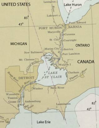
Figure 1. Study area showing Lake St. Clair in the Great Lakes Waterway. (Base map from NOAA Chart 14500, Great Lakes: Lake Champlain to Lake of the Woods, 2000 (ed.), 1:500,000.)
Purpose and Scope
This report describes the movement of drifting buoys and flow velocity as a function of depth for selected points on Lake St. Clair from August 12-15, 2002. Ancillary wind and water-level data during the deployments also are shown. This information provides a basis for identifying circulation patterns and refining the calibration of a hydrodynamic model of the waterway that includes Lake St. Clair (Holtschlag and Koschik, 2002). The field study was conducted to help identify source areas to public water intakes on the waterway. Computer animations and images were developed to help visualize the data. The animations and images can be accessed through the Internet with a standard web browser and readily available plugin.
Previous Investigations
Schwab and others (1989) used three different types of measurements to investigate circulation patterns on Lake St. Clair. These measurements included use of an array of fixed current meters, seven synoptic ship-based measurements of currents, and four experiments using satellite-tracking of drifting buoys. Drifting buoy studies of St. Clair River (Holtschlag and Aichele, 2001, http://mi.water.usgs.gov/pubs/OF/OF01-17/) and Detroit River (Holtschlag and Aichele, 2002, http://mi.water.usgs.gov/pubs/OF/OF02-1/), were developed using similar equipment and techniques as those described in this report. The distribution of flows through branches in St. Clair River and Detroit River, including the distributaries in the St. Clair River delta, are described by Holtschlag and Koschik (2001). A hydrodynamic flow model of the St. Clair - Detroit River Waterway, including Lake St. Clair, is described by Holtschlag and Koschik (2002).
Acknowledgements
This report was developed by USGS in cooperation with Michigan Department of Environmental Quality, Source Water Assessment Program, directed by Bradley B. Brogren; Detroit Water and Sewerage Department's Water Quality Division, managed by Pamela Turner; and the American Water Works Association Research Foundation's Christopher Rayburn, who directs the Research Management Department. Don A. James and C. Edward Lipinski, of the USGS Field Office in Grayling, Michigan, provided technical assistance with the ADCP equipment and helped deploy, locate, and retrieve the buoys. Buoys used in the deployment were obtained through the USGS NASQAN (National Streamflow Quality Accounting Network) program with the help of Richard P. Hooper, Northborough, Massachusetts. The USGS - Great Lakes Science Center (Biological Resources Discipline), Ann Arbor, Michigan, provided the use of their research vessel Dragonfly for the buoy deployment and ADCP surveys.
METHODS
Twelve drifting buoys were released southwest of where South Channel, St. Clair Flats Canal, and St. Clair Cutoff flow into Lake St. Clair (Figure 2, Figure 3). This location was selected because the combined flows from these branches account for about 41.3 percent of the total flow through Lake St. Clair (Holtschlag and Koschik, 2001) and because of its location on the navigational channel. The transect is located about 15.5 miles northeast of the upper limit of Detroit River.
Figure 2. Locations of gaging stations and streams tributary to Lake St. Clair.
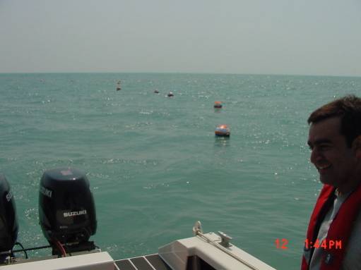
Figure 3. Transect of drifting buoys on the navigational channel of Lake St. Clair.
Buoy and Drogue Characteristics
The buoys (Figure 4) are surface drifters that were originally designed for extended deployments in ocean environments by Clearwater Instrumentation®, Inc. The buoys are formed by joining two fiberglass hemispheres around a rubber oring with a metal clamp. The resulting spherical buoys are about 16 inches in diameter and weigh about 35 pounds. For Lake St. Clair deployments, the buoys were equipped with GARMIN® GPS 12 receivers, which were oriented horizontally, facing upward, near the top of the buoys. The GPS receivers were configured to internally record their positions at 3-minute intervals. These receivers have a rated positional accuracy (root mean square error) of 49 ft (Garmin Corporation, 1999, p. 52). Original GPS, telemetry, and power supplies were removed from the buoys for these deployments. Metal reflective tape was wrapped around the center of the buoys' upper hemisphere to enhance their visibility.
To provide a power supply for deployments that exceeded normal battery life of the GPS receivers, an exterior 8.0 ampere-hour 12-volt battery, wired for 6-volts, replaced the standard four internal AA batteries. The batteries were placed near the bottoms of the spheres for ballast. Styrofoam® was packed around the GPS recievers and batteries inside the buoys to secure their positions and to help the buoys maintain their buoyancy in case of leaks.
Drogues, which act like sea anchors, were suspended below the buoys to increase the sensitivity of buoy movements to currents across the drogued interval and to reduce the direct effect of winds on buoy movements. Drogues were formed by two vertically-oriented planes set at right angles to one another along a weighted line (Figure 4). Each plane was constructed of nylon fabric that was about 18 inches tall and 30 inches wide. The fabric was stretched between 1-inch PVC tubing. A weight of about 3 pounds was fastened to the bottom of the drogues to help maintain the vertical orientation of the drogues. Drogues were set at one of two depth intervals to help assess possible vertical variations in velocity. Eight buoys were drogued through an interval of 1-4 feet, and four buoys were drogued through an interval of 4-7 feet below the water surface.
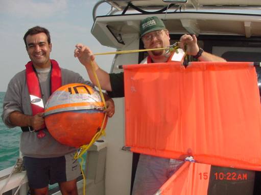
Figure 4. Drifting buoys and drogues deployed on Lake St. Clair.
Acoustic Doppler Current Profiler Survey of Lake St. Clair
An ADCP (acoustic Doppler current profiler) survey was conducted during the drifting buoy deployment on Lake St. Clair to provide an overview of the flow velocity field through which the buoys were drifting and to describe possible velocity variations with depth. The R.D. Instruments® 600 kilohertz Workhorse "Rio Grande" ADCP (Figure 5) used in the survey was mounted on a small raft, which was tethered to the side of the boat, similar to (Figure 6, Figure 7).
Survey points were located across a regular grid (Table 1) within the lake where currents were likely to directly effect buoy movements. Grid points were located at approximately 1.7 minute intervals of latitude (1.92 mile intervals) and 2.5 minute intervals of longitude (2.13 miles intervals). At each grid point, the boat was held in a nearly fixed position and the ADCP was operated for a period of about 10 minutes. During these measurement periods, the ADCP obtained point velocities at 0.4-second intervals and 0.5-meter depth intervals through the water column starting 1.0 meter below the water surface. In addition to velocities, the ADCP unit sensed the lake bottom, which provided the reference for the flow velocities. The configuration file for the ADCP survey (Appendix A) specified a magnetic delination of 7 degrees west of north, among other parameters.
Instantaneous water velocity measurements were highly variable and showed little consistency in speed or direction (Table 2). The variability is associated with the generally low water velocities in the lake and surface waves assoicated with wind, which caused significant movement of the raft carrying the ADCP unit. Averaging the instantaneous velocities at each depth over the measurement period removed much of the variability and identified differences in water velocity with depth (Figure 8).
Table 1. Measured locations of ADCP grid points and ADCP file names.
| Grid point identifier | Latitude | Longitude | Way Point | Starting date and time |
Link to ADCP file ASCII files |
|
|---|---|---|---|---|---|---|
| Report | Field | |||||
| A6 | 116 | 42° 23' 20.3" | 82° 52' 28.7" | 198 | 8/14/02 13:13 | LscGrid116(520KB) |
| A7 | 115 | 42° 21' 39.9" | 82° 52' 29.7" | 197 | 8/14/02 12:55 | LscGrid115(416KB) |
| B5 | 006 | 42° 25' 01.7" | 82° 50' 00.3" | 241 | 8/15/02 15:36 | LscGrid006(584KB) |
| B6 | 007 | 42° 23' 20.1" | 82° 49' 58.9" | 199 | 8/14/02 13:31 | LscGrid007(592KB) |
| B7 | 008 | 42° 21' 40.3" | 82° 50' 00.3" | 200 | 8/14/02 13:53 | LscGrid008(508KB) |
| B8 | 009 | 42° 20' 00.7" | 82° 49' 58.8" | 196 | 8/14/02 12:34 | LscGrid009(400KB) |
| C1 | 012 | 42° 31' 40.6" | 82° 47' 30.5" | 165 | 8/13/02 14:19 | LscGrid012(496KB) |
| C2 | 013 | 42° 30' 01.0" | 82° 47' 31.6" | 164 | 8/13/02 13:56 | LscGrid013(564KB) |
| C3 | 014 | 42° 28' 19.7" | 82° 47' 30.7" | 163 | 8/13/02 13:33 | LscGrid014(560KB) |
| C4 | 015 | 42° 26' 39.9" | 82° 47' 30.4" | 162 | 8/13/02 13:08 | LscGrid015(612KB) |
| C5 | 016 | 42° 24' 59.5" | 82° 47' 29.5" | 161 | 8/13/02 12:45 | LscGrid016(612KB) |
| C6 | 017 | 42° 23' 20.4" | 82° 47' 30.9" | 240 | 8/15/02 15:12 | LscGrid017(580KB) |
| C7 | 018 | 42° 21' 39.8" | 82° 47' 29.6" | 201 | 8/14/02 14:13 | LscGrid018(564KB) |
| C8 | 019 | 42° 20' 00.1" | 82° 47' 30.1" | 195 | 8/14/02 12:12 | LscGrid019(476KB) |
| D1 | 022 | 42° 31' 40.4" | 82° 45' 00.3" | 91 | 8/12/02 15:33 | LscGrid022(324KB) |
| D2 | 023 | 42° 30' 00.6" | 82° 44' 59.7" | 92 | 8/12/02 15:54 | LscGrid023(384KB) |
| D3 | 024 | 42° 28' 20.4" | 82° 45' 00.0" | 125 | 8/12/02 17:30 | LscGrid024(464KB) |
| D4 | 025 | 42° 26' 40.1" | 82° 44' 58.2" | 126 | 8/12/02 17:50 | LscGrid025(364KB) |
| D5 | 026 | 42° 25' 01.5" | 82° 45' 01.5" | 160 | 8/13/02 12:17 | LscGrid026(796KB) |
| D6 | 027 | 42° 23' 21.3" | 82° 45' 00.0" | 239 | 8/15/02 14:48 | LscGrid027(620KB) |
| D7 | 028 | 42° 21' 40.1" | 82° 45' 00.1" | 202 | 8/14/02 14:31 | LscGrid028(544KB) |
| D8 | 029 | 42° 20' 00.5" | 82° 45' 01.0" | 193 | 8/14/02 11:51 | LscGrid029(544KB) |
| E1 | 032 | 42° 31' 40.3" | 82° 42' 30.5" | 90 | 8/12/02 15:15 | LscGrid032(248KB) |
| E2 | 033 | 42° 29' 58.3" | 82° 42' 32.0" | 84 | 8/12/02 14:54 | LscGrid033(436KB) |
| E3 | 034 | 42° 28' 20.4" | 82° 42' 29.6" | 124 | 8/12/02 17:13 | LscGrid034(380KB) |
| E4 | 035 | 42° 26' 40.8" | 82° 42' 30.0" | 128 | 8/12/02 18:09 | LscGrid035(400KB) |
| E5 | 036 | 42° 25' 00.0" | 82° 42' 29.7" | 159 | 8/13/02 11:54 | LscGrid036(576KB) |
| E6 | 037 | 42° 23' 20.8" | 82° 42' 29.1" | 238 | 8/15/02 14:21 | LscGrid037(664KB) |
| E7 | 038 | 42° 21' 40.4" | 82° 42' 30.4" | 203 | 8/14/02 14:47 | LscGrid038(552KB) |
| E8 | 039 | 42° 20' 03.6" | 82° 42' 25.2" | 190 | 8/13/02 11:09 | LscGrid039(636KB) |
| F2 | 043 | 42° 30' 00.2" | 82° 39' 59.4" | 231 | 8/15/02 11:17 | LscGrid043(500KB) |
| F3 | 044 | 42° 28' 19.2" | 82° 39' 58.6" | 230 | 8/15/02 10:52 | LscGrid044(580KB) |
| F4 | 045 | 42° 26' 40.8" | 82° 40' 00.3" | 157 | 8/13/02 11:09 | LscGrid045(600KB) |
| F5 | 046 | 42° 25' 00.7" | 82° 40' 00.0" | 158 | 8/13/02 11:32 | LscGrid046(568KB) |
| F6 | 047 | 42° 23' 20.4" | 82° 40' 01.1" | 237 | 8/15/02 13:52 | LscGrid047(720KB) |
| F7 | 048 | 42° 21' 40.2" | 82° 40' 00.4" | 204 | 8/14/02 15:06 | LscGrid048(516KB) |
| G2 | 053 | 42° 29' 59.3" | 82° 37' 30.3" | 232 | 8/15/02 11:43 | LscGrid053(516KB) |
| G3 | 054 | 42° 28' 19.7" | 82° 37' 29.5" | 233 | 8/15/02 12:18 | LscGrid054(468KB) |
| G4 | 055 | 42° 26' 39.9" | 82° 37' 28.1" | 234 | 8/15/02 12:45 | LscGrid055(592KB) |
| G5 | 056 | 42° 24' 59.6" | 82° 37' 30.4" | 235 | 8/15/02 13:09 | LscGrid056(644KB) |
| G6 | 057 | 42° 23' 19.6" | 82° 37' 30.8" | 236 | 8/15/02 13:31 | LscGrid057(552KB) |
Figure 5. An R.D. Instruments, Inc., 600-kilohertz Workhorse "Rio Grande" acoustic Doppler current profiler.
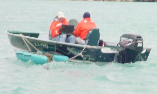
Figure 6. ADCP fastened between floats of a small pontoon and tethered to a boat for velocity measurements.
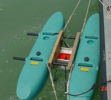
Figure 7. ADCP mounted between pontoons on raft.
Movie clip showing ADCP movement during velocity measurement (MPEG 478KB).
Table 2. Distribution of instantaneous water velocities by depth measured using an ADCP at 0.4 second intervals near grid point D6 on Lake St. Clair from August 12, 2002 at 12:17 to 12:31 EDT (Eastern Daylight Time).
|
Note: Unlike a standard wind chart, the graphs below indicate the direction to which water is flowing, rather than the direction from which water is originating. |
|
|
|
|
|
|
|
|
|
|
|
|
|
|
|
|
|
|
(Note: Grid point D6 is shown on figure 2.)
Figure 8. Temporally averaged ADCP velocities with depth for grid point D6 on Lake St. Clair. (Note: The green plane identifies the lake bottom. The velocity vector projected on the green plane represents a vertically and temporally averaged velocity. The temporally averaged velocity vectors are plotted at their depth coordinate. The view is orthogonal to the projected velocity, which is 222 degrees clockwise from true north and at an altitude of 20 degrees above the horizon. Grid points are identified on Figure 2.)
Ancillary Data
Water Levels
Water-level data were obtained from three water-level gaging stations on Lake St. Clair (Figure 2). Two stations operated by the National Oceanic and Atmospheric Administration (NOAA) are located in Michigan (MI), and one station is operated by the Canadian Hydrographic Service (CHS) is located in Ontario (ON). Water levels generally ranged less than 0.2 ft during the buoy deployment (Figure 9). Although average water levels were nearly constant, there is a slight downward trend. Water levels at Windmill Point, Michigan station are lower than the other two stations because of the influence of Detroit River.
Figure 9. Water levels during the buoy deployment on Lake St. Clair in the Great Lakes Waterway.
Flows
Water-level data from four NOAA gaging stations on St. Clair River were used with regression equations (John Koschik, U.S. Army Corps of Engineers, written commun., 2002) and average flow conditions on the major tributaries to compute the expected inflow to Lake St. Clair. The four gaging stations included: Dunn Paper, DP, (station 9014096), Mouth of Black River, MBR, (station 9014090), Dry Dock, DD, (station 9014087), and St. Clair State Police, SCSP, (station 9014080). Six-minute water-level data from 07:30 on August 12, 2002, to 23:54 on August 15, 2002, were used in the computations, because of missing water-level data at the Dunn Paper station during the morning of August 12, 2002.
The average of six-minute flow values were computed by use of the three regression equations that relate discharge (Q, in cubic meters per second) to stage (water level, in meters) and fall (the difference between water levels at two gaging stations) as:
| (1) | |
| (2) | |
| (3) |
After converting units, the above equations resulted in estimates of 170,600, 174,000, and 170,800 ft3/s, respectively, for an average flow of 171,800 ft3/s. After accounting for average inflows from major tributaries, the distribution of outflows in branches of St. Clair River computed based on the equations developed by Holtschlag and Koschik (2001) is shown in Figure 10.
Figure 10. Flow schematic for St. Clair River and Lake St. Clair from August 12-15, 2002.
Winds
Wind data were obtained from the Coastal-Marine Automated Network (C-MAN) station LSCM4 on Lake St. Clair (Figure 11). Data for this station, which is operated by the National Data Buoy Center, can be access through the Internet at the URL: http://www.ndbc.noaa.gov/station_page.php?station=lscm4. During the August 12-15, 2002 deployment, winds were generally a moderate breeze, a Beaufort scale force 4 condition, from the south, southwest (Figure 12). At times, wave heights exceeded 3.5 feet, and white caps were numerous.
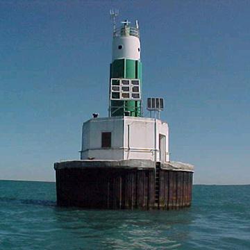
Figure 11. Lake St. Clair weather station LSCM4, which is mounted on Lake St. Clair Light.
Figure 12. Wind conditions on Lake St. Clair from August 12-15, 2002. (Perimeter shows the angle from which winds were originating, in degrees).
RESULTS
Drifting Buoy Deployment
Twelve drifting buoys were initially deployed along a transect between navigational buoys separated by about 800 ft in the northcentral part of Lake St. Clair just south of the St. Clair River delta and 15.5 mi northeast of Detroit River (Animation). During their 74-hour deployment between August 12-15, 2002, the buoys generally drifted toward the south, making unsteady progress toward the middle of the lake, for a maximum drift distance of about 7.5 miles. In the first two days of the deployment, the eight shallow buoys, drogued at 1-4 ft, and the four deep buoys, drogued at 4-7 ft, tended to form two distinct clusters. During this period, the deep buoys tended to drift ahead (south) and to the west of the shallow buoys. On the last day of the deployment, however, the most southernly group of shallow buoys joined the deeper buoy cluster in the south. Meanwhile, the shallow buoys in the northern part of their cluster, changed direction and drifted back toward the north and east. At the end of the deployment, 4.8 mi separated the most southerly (deep) buoy and the most northeasterly (shallow) buoy. Buoys were retrieved before reaching Detroit River because engine problems onboard the Dragonfly shortened the deployment.
ADCP Velocity Survey
In addition to the buoy deployments, ADCP vertical velocities were surveyed at 41 grid points within the lake that spanned the area through which the buoys drifted (Animation). The vertically and temporally averaged water velocities at the grid points ranged from 0.03 to 0.89 ft/s (feet per second), with the greatest measured velocity occurring on the navigational channel near the deployment transect. In general, water speeds were greater at mid-depths than near the water surface (Figure 13), during conditions in which wind direction opposed the general flow direction. The variability of water direction decreased with depth below the water surface, and tended to have a larger westerly component with increasing depth (Figure 14).
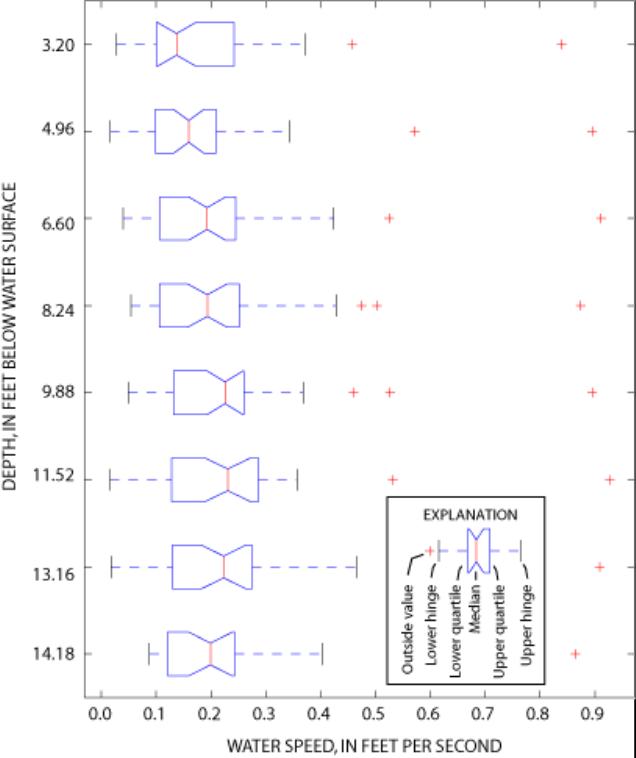
Figure 13. Variation of water speed with depth at ADCP grid point D6 on Lake St. Clair.
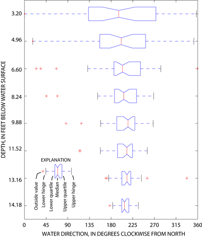
Figure 14. Variation of water direction with depth at ADCP grid point D6 on Lake St. Clair.
Visualization
A web page was developed to animate buoy movements using LiveMotion 2, by Adobe® Corporation (Animation). Background images for the animations were scanned from recreational charts (National Oceanic and Atmospheric Administration, 1999) published at a scale 1:120,000. The pixel coordinates of the scanned images were registered with positional information on the maps to facilitate plotting of buoy locations. Buoy locations were generally included at 30-minute intervals based on GPS data. Between measured locations, buoy positions are interpolated by use of a Bezier curve. Pairs of Macromedia® Flash file format (SWF) and hypertext markup language (HTML) files were created to display the animation through the Internet. Motion controls are provided on the animations to stop, play continuously or frame by frame, and restart the animation.
In addition to the animations, the web page contains links at grid points to images of three-dimensional plots of velocity vectors with depth (like Figure 8). For each grid point, a three by three array of views is provided. The views include three views at different azimuts that are orthogonal to the direction of the minimum, average, and maximum velocity azimuth, and at three views at altitudes of 10, 20, and 30 degrees above the horizon.
SUMMARY
Twelve buoys equipped with GPS receivers were deployed in the northcentral part of Lake St. Clair in the Great Lakes Waterway between August 12-15, 2002. Eight buoys were drogued at a shallow depth interval, 1-4 ft, and four were drogued at a deep depth interval, 4-7 ft, intervals to assess the possible variation of velocity with water depth and to reduce the direct effect of wind on buoy movements. During their 74-hour deployment, the buoys generally drifted toward the south, making unsteady progress toward the middle of the lake in route to Detroit River. Acoustic Doppler current profiler (ADCP) velocity surveys were obtained at 41 points in Lake St. Clair that spanned the region through which the buoys drifted. Results of these deployments were animated to facilitate visualization of the results and further study. Ancillary velocity, water level, and wind measurements provide data to support future interpretations of the results.
Animation - Lake St. Clair ADCP Survey and Buoy Deployment
REFERENCES CITED
Appendix A. Configuration file for ADCP velocity profiles on Lake St. Clair.
[RDI WinRiver Configuaration File]
Version=10.03.000
[Subsection]
Use All Ensembles=YES
First Ensemble=0
Last Ensemble=131071
[Offsets]
ADCP Transducer Depth [m]=0.152392563
Magnetic Variation [deg]=-7
Heading Offset [deg]=0
One Cycle K=0
One Cycle Offset=0
Two Cycle K=0
Two Cycle Offset=0
[Processing]
Speed of Sound Correction=0
Salinity [ppt]=0
Fixed Speed Of Sound [m/s]=1500
Mark Below Botom Bad=YES
Backscatter Type=0
Intensity Scale [dB/cts]=0.43
Absorption [dB/m]=0.139
Projection Angle [deg]=0
Cross Area Type=2
Use 3 Beam Solution For BT=YES
Use 3 Beam Solution For WT=NO
BT Error Velocity Threshold [m/s]=0.100579092
WT Error Velocity Threshold [m/s]=1.499542822
BT Up Velocity Threshold [m/s]=10
WT Up Velocity Threshold [m/s]=10
Fish Intensity Threshold [counts]=50
Near Zone Distance=2.099969521
[Discharge]
Top Discharge Estimate=0
Bottom Discharge Estimate=0
Power Curve Coef=0.1667
Cut Top Bins=0
Cut Bins Above Sidelobe=0
River Left Edge Type=0
Left Edge Slope Coeff=0.5
River Right Edge Type=0
Right Edge Slope Coeff=0.5
Shore Pings Avg=10
[Edge Estimates]
Begin Shore Distance=0
Begin Left Bank=YES
End Shore Distance=0
[Depth Sounder]
Use Depth Sounder In Processing=NO
Depth Sounder Transducer Depth [m]=0
Depth Sounder Transducer Offset [m]=0
Depth Sounder Correct Speed of Sound=NO
Depth Sounder Scale Factor=1
[GPS]
GPS Time Delay [s]=0
[Recording]
Filename Prefix=lsc815
Output Directory=D:\Projects\Current\SCD\LSC\ADCP\Aug15\
GPS Recording=NO
DS Recording=NO
Maximum File Size [MB]=0
Comment #1=Lake St. Clair at Grid Point 33
Comment #2=Don James, Atiq Syed, Greg Kennedy, and Dave Holtschlag
Next Transect Number=0
[Commands]
[Wizard Commands]
BX170
WF25
WM1
WN34
WS50
WV170
TP000020
[Wizard Info]
ADCP Type=1
Use Radio Modem=NO
Use GPS=NO
Use Depth Sounder=NO
Max Water Depth=13.715330692
Max Water Speed=0.609570253
Max Boat Speed=0.609570253
Material=2
Water Mode=0
Beam Angle [deg]=20
[Charts]
East Velocity Minimum=-0.609570253
East Velocity Maximum=0.609570253
North Velocity Minimum=-0.609570253
North Velocity Maximum=0.609570253
Up Velocity Minimum=-0.121914051
Up Velocity Maximum=0.121914051
Error Velocity Minimum=-0.121914051
Error Velocity Maximum=0.121914051
Velocity Magnitude Minimum=0
Velocity Magnitude Maximum=0.609570253
Velocity Direction Minimum=0
Velocity Direction Maximum=360
Projected Velocity Minimum=-0.609570253
Projected Velocity Maximum=0.609570253
Depth Minimum=0
Depth Maximum=13.715330692
East Displacement Minimum=-2.320226523
East Displacement Maximum=48.724756987
North Displacement Minimum=-10.652557858
North Displacement Maximum=223.703715009
Intensity Minimum=40
Intensity Maximum=255
Backscatter Minimum=0
Backscatter Maximum=255
Correlation Minimum=0
Correlation Maximum=128
Discharge Minimum=-5.000023069
Discharge Maximum=5.000023069
Heading Minimum=0
Heading Maximum=360
Pitch Roll Minimum=-10
Pitch Roll Maximum=10
Water Speed Minimum=0
Water Speed Maximum=0.609570253
Boat Speed Minimum=0
Boat Speed Maximum=0.609570253